LING YANG, Peking University, China

ZHILONG ZHANG∗ , Peking University, China

YANG SONG, OpenAI, USA

SHENDA HONG, Peking University, China

RUNSHENG XU, University of California, Los Angeles, USA

YUE ZHAO, Carnegie Mellon University, USA

WENTAO ZHANG, Peking University, China

BIN CUI, Peking University, China

MING-HSUAN YANG† , University of California at Merced, USA

Diffusion models have emerged as a powerful new family of deep generative models with record-breaking performance in many applications, including image synthesis, video generation, and molecule design. In this survey, we provide an overview of the rapidly expanding body of work on diffusion models, categorizing the research into three key areas: efficient sampling, improved likelihood estimation, and handling data with special structures. We also discuss the potential for combining diffusion models with other generative models for enhanced results. We further review the wide-ranging applications of diffusion models in fields spanning from computer vision, natural language processing, temporal data modeling, to interdisciplinary applications in other scientific disciplines. This survey aims to provide a contextualized, in-depth look at the state of diffusion models, identifying the key areas of focus and pointing to potential areas for further exploration. Github: https://github.com/YangLing0818/Diffusion-Models-Papers-Survey-Taxonomy.

CCS Concepts: • Computing methodologies → Computer vision tasks; Natural language generation; Machine learning approaches.

Additional Key Words and Phrases: Generative Models, Diffusion Models, Score-Based Generative Models, Stochastic Differential Equations

### ACM Reference Format:

Ling Yang, Zhilong Zhang, Yang Song, Shenda Hong, Runsheng Xu, Yue Zhao, Wentao Zhang, Bin Cui, and Ming-Hsuan Yang. 2023. Diffusion Models: A Comprehensive Survey of Methods and Applications. 1, 1 (December 2023), 58 pages. https://doi.org/10.1145/ 3626235

∗Contributed equally.

<sup>†</sup>Wentao Zhang, Bin Cui, and Ming-Hsuan Yang are corresponding authors.

Authors' addresses: Ling Yang, Peking University, China, yangling0818@163.com; Zhilong Zhang, Peking University, China, zhilong.zhang@bjmu.edu.cn; Yang Song, OpenAI, USA, songyang@openai.com; Shenda Hong, Peking University, China, hongshenda@pku.edu.cn; Runsheng Xu, University of California, Los Angeles, USA, rxx3386@ucla.edu; Yue Zhao, Carnegie Mellon University, USA, zhaoy@cmu.edu; Wentao Zhang, Peking University, China, wentao.zhang@pku.edu.cn; Bin Cui, Peking University, China, bin.cui@pku.edu.cn; Ming-Hsuan Yang, University of California at Merced, USA, mhyang@ucmerced.edu.

Permission to make digital or hard copies of all or part of this work for personal or classroom use is granted without fee provided that copies are not made or distributed for profit or commercial advantage and that copies bear this notice and the full citation on the first page. Copyrights for components of this work owned by others than ACM must be honored. Abstracting with credit is permitted. To copy otherwise, or republish, to post on servers or to redistribute to lists, requires prior specific permission and/or a fee. Request permissions from permissions@acm.org.

<sup>© 2023</sup> Association for Computing Machinery.

Manuscript submitted to ACM

# Contents

| Abstract |  | 1 |
| --- | --- | --- |
| Contents |  | 2 |
| 1 | Introduction | 3 |
| 2 | Foundations of Diffusion Models | 5 |
| 2.1 | Denoising Diffusion Probabilistic Models (DDPMs) | 5 |
| 2.2 | Score-Based Generative Models (SGMs) | 8 |
| 2.3 | Stochastic Differential Equations (Score SDEs) | 9 |
| 3 | Diffusion Models with Efficient Sampling | 10 |
| 3.1 | Learning-Free Sampling | 10 |
| 3.1.1 | SDE Solvers | 10 |
| 3.1.2 | ODE solvers | 12 |
| 3.2 | Learning-Based Sampling | 13 |
| 3.2.1 | Optimized Discretization | 13 |
| 3.2.2 | Truncated Diffusion | 14 |
| 3.2.3 | Knowledge Distillation | 14 |
| 4 | Diffusion Models with Improved Likelihood | 14 |
| 4.1 | Noise Schedule Optimization | 14 |
| 4.2 | Reverse Variance Learning | 15 |
| 4.3 | Exact Likelihood Computation | 16 |
| 5 | Diffusion Models for Data with Special Structures | 17 |
| 5.1 | Discrete Data | 17 |
| 5.2 | Data with Invariant Structures | 17 |
| 5.3 | Data with Manifold Structures | 18 |
| 5.3.1 | Known Manifolds | 18 |
| 5.3.2 | Learned Manifolds | 18 |
| 6 | Connections with Other Generative Models | 19 |
| 6.1 | Large Language Models and Connections with Diffusion Models | 19 |
| 6.2 | Variational Autoencoders and Connections with Diffusion Models | 20 |
| 6.3 | Generative Adversarial Networks and Connections with Diffusion Models | 21 |
| 6.4 | Normalizing Flows and Connections with Diffusion Models | 22 |
| 6.5 | Autoregressive Models and Connections with Diffusion Models | 23 |
| 6.6 | Energy-based Models and Connections with Diffusion Models | 24 |
| 7 | Applications of Diffusion Models | 24 |
| 7.1 | Unconditional and Conditional Diffusion Models | 24 |
| 7.1.1 | Conditioning Mechanisms in Diffusion Models | 25 |
| 7.1.2 | Diffusion with DPO/RLHF | 25 |
| 7.1.3 | Condition Diffusion on Labels and Classifiers | 27 |
| 7.1.4 | Condition Diffusion on Texts, Images, and Semantic Maps | 27 |
| 7.1.5 | Condition Diffusion on Graphs | 27 |

| 7.2 | Computer Vision | 27 |
| --- | --- | --- |
| 7.2.1 | Image Super Resolution, Inpainting, Restoration, Translation, and Editing | 27 |
| 7.2.2 | Semantic Segmentation | 29 |
| 7.2.3 | Video Generation | 29 |
| 7.2.4 | Generating Data from Diffusion Models | 29 |
| 7.2.5 | Point Cloud Completion and Generation | 29 |
| 7.2.6 | Anomaly Detection | 31 |
| 7.3 | Natural Language Generation | 31 |
| 7.4 | Multi-Modal Generation | 32 |
| 7.4.1 | Text-to-Image Generation | 32 |
| 7.4.2 | Scene Graph-to-Image Generation | 34 |
| 7.4.3 | Text-to-3D Generation | 34 |
| 7.4.4 | Text-to-Motion Generation | 37 |
| 7.4.5 | Text-to-Video Generation | 38 |
| 7.4.6 | Text-to-Audio Generation | 38 |
| 7.5 | Temporal Data Modeling | 40 |
| 7.5.1 | Time Series Imputation | 40 |
| 7.5.2 | Time Series Forecasting | 40 |
| 7.5.3 | Waveform Signal Processing | 41 |
| 7.6 | Robust Learning | 41 |
| 7.7 | Interdisciplinary Applications | 41 |
| 7.7.1 | Drug Design and Life Science | 41 |
| 7.7.2 | Material Design | 42 |
| 7.7.3 | Medical Image Reconstruction | 43 |
| 8 | Future Directions | 43 |
| Revisiting Assumptions |  | 43 |
|  | Theoretical Understanding | 44 |
| Latent Representations |  | 44 |
|  | AIGC and Diffusion Foundation Models | 44 |
| 9 Conclusion |  | 44 |
| References |  | 44 |

# 1 INTRODUCTION

Diffusion models [111, 275, 280, 285] have emerged as the new state-of-the-art family of deep generative models. They have broken the long-time dominance of generative adversarial networks (GANs) [88] in the challenging task of image synthesis [60, 111, 280, 285] and have also shown potential in a variety of domains, ranging from computer vision [4, 15, 25, 29, 112, 114, 145, 149, 171, 194, 206, 225, 257, 259, 315, 354, 355, 379, 389], natural language processing [9, 117, 175, 264, 361], temporal data modeling [3, 39, 159, 249, 291, 335], multi-modal modeling [10, 243, 255, 258, 386],

![](_page_3_Figure_1.jpeg)

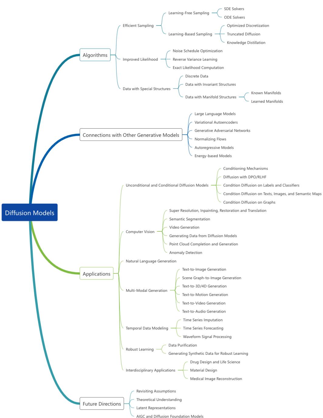
Fig. 1. Taxonomy of diffusion models variants (in Sections 3 to 5), connections with other generative models (in Section 6), applications of diffusion models (in Section 7), and future directions (in Section 8).

robust machine learning [23, 33, 144, 308, 357], to interdisciplinary applications in fields such as computational chemistry [5, 115, 133, 166, 169, 196, 327] and medical image reconstruction [31, 47–49, 53, 202, 230, 284, 328].

Numerous methods have been developed to improve diffusion models, either by enhancing empirical performance [214, 277, 281] or by extending the model's capacity from a theoretical perspective [187, 188, 279, 285, 371]. Over the past two years, the body of research on diffusion models has grown significantly, making it increasingly challenging for new researchers to stay abreast of the recent developments in the field. Additionally, the sheer volume of work can obscure major trends and hinder further research progress. This survey aims to address these problems by providing a comprehensive overview of the state of diffusion model research, categorizing various approaches, and highlighting key advances. We hope this survey to serve as a helpful entry point for researchers new to the field while providing a broader perspective for experienced researchers.

In this paper, we first explain the foundations of diffusion models (Section 2), providing a brief but self-contained introduction to three predominant formulations: denoising diffusion probabilistic models (DDPMs) [111, 275], scorebased generative models (SGMs) [280, 281], and stochastic differential equations (Score SDEs) [141, 279, 285]. Key to all these approaches is to progressively perturb data with intensifying random noise (called the "diffusion" process), then successively remove noise to generate new data samples. We clarify how they work under the same principle of diffusion and explain how these three models are connected and can be reduced to one another.

Next, we present a taxonomy of recent research that maps out the field of diffusion models, categorizing it into three key areas: efficient sampling (Section 3), improved likelihood estimation (Section 4), and methods for handling data with special structures (Section 5), such as relational data, data with permutation/rotational invariance, and data residing on manifolds. We further examine the models by breaking each category into more detailed sub-categories, as illustrated in Fig. 1. In addition, we discuss the connections of diffusion models to other deep generative models (Section 6), including variational autoencoders (VAEs) [156, 252], generative adversarial networks (GANs) [88], normalizing flows [62, 64, 226, 254], autoregressive models [302], and energy-based models (EBMs) [165, 283]. By combining these models with diffusion models, researchers have the potential to achieve even stronger performance.

Following that, our survey reviews six major categories of application that diffusion models have been applied to in the existing research (Section 7): computer vision, natural language process, temporal data modeling, multi-modal learning, robust learning, and interdisciplinary applications. For each task, we provide a definition, describe how diffusion models can be employed to address it and summarize relevant previous work. We conclude our paper (Sections 8 and 9) by providing an outlook on possible future directions for this exciting new area of research.

### 2 FOUNDATIONS OF DIFFUSION MODELS

Diffusion models are a family of probabilistic generative models that progressively destruct data by injecting noise, then learn to reverse this process for sample generation. We present the intuition of diffusion models in Fig. 2. Current research on diffusion models is mostly based on three predominant formulations: denoising diffusion probabilistic models (DDPMs) [111, 214, 275], score-based generative models (SGMs) [280, 281], and stochastic differential equations (Score SDEs) [279, 285]. We give a self-contained introduction to these three formulations in this section, while discussing their connections with each other along the way.

### 2.1 Denoising Diffusion Probabilistic Models (DDPMs)

A denoising diffusion probabilistic model (DDPM) [111, 275] makes use of two Markov chains: a forward chain that perturbs data to noise, and a reverse chain that converts noise back to data. The former is typically hand-designed with

![](_page_5_Figure_1.jpeg)

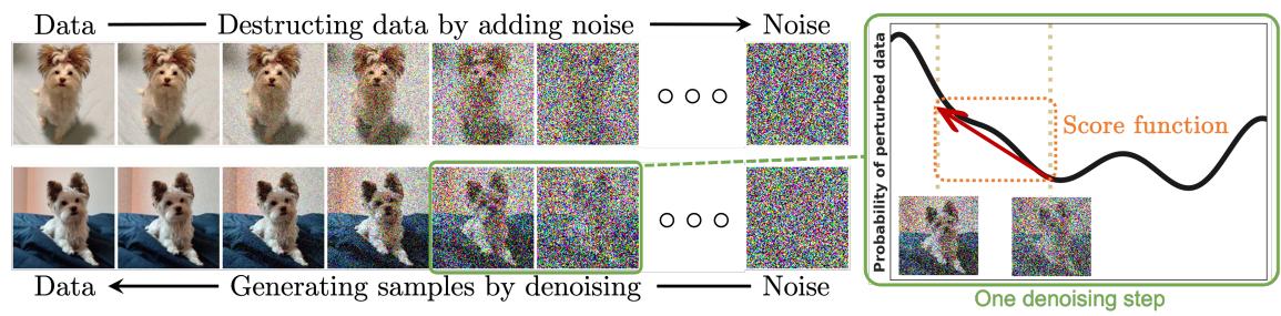
Fig. 2. Diffusion models smoothly perturb data by adding noise, then reverse this process to generate new data from noise. Each denoising step in the reverse process typically requires estimating the score function (see the illustrative figure on the right), which is a gradient pointing to the directions of data with higher likelihood and less noise.

the goal to transform any data distribution into a simple prior distribution (e.g., standard Gaussian), while the latter Markov chain reverses the former by learning transition kernels parameterized by deep neural networks. New data points are subsequently generated by first sampling a random vector from the prior distribution, followed by ancestral sampling through the reverse Markov chain [158].

Formally, given a data distribution x0 ∼ (x0), the forward Markov process generates a sequence of random variables x1, x2 . . . x with transition kernel (x | x−1). Using the chain rule of probability and the Markov property, we can factorize the joint distribution of x1, x2 . . . x conditioned on x0, denoted as (x1, . . . , x | x0), into

$$q(\mathbf{x}_{1},\ldots,\mathbf{x}_{T}\mid\mathbf{x}_{0})=\prod_{t=1}^{T}q(\mathbf{x}_{t}\mid\mathbf{x}_{t-1}).\tag{1}$$

In DDPMs, we handcraft the transition kernel (x | x−1) to incrementally transform the data distribution (x0) into a tractable prior distribution. One typical design for the transition kernel is Gaussian perturbation, and the most common choice for the transition kernel is

$$q({\bf x}_{t}\mid{\bf x}_{t-1})={\cal N}({\bf x}_{t};\sqrt{1-\beta_{t}}{\bf x}_{t-1},\beta_{t}{\bf I}),\tag{2}$$

where ∈ (0, 1) is a hyperparameter chosen ahead of model training. We use this kernel to simply our discussion here, although other types of kernels are also applicable in the same vein. As observed by Sohl-Dickstein et al. (2015) [275], this Gaussian transition kernel allows us to marginalize the joint distribution in Eq. (1) to obtain the analytical form of (x | x0) for all ∈ {0, 1, · · · , }. Specifically, with B 1 − and ¯ B Î =0 , we have

$$q({\bf x}_{t}\mid{\bf x}_{0})={\cal N}({\bf x}_{t};\sqrt{\tilde{\alpha}_{t}}{\bf x}_{0},(1-\tilde{\alpha}_{t}){\bf I}).\tag{3}$$

Given x0, we can easily obtain a sample of x by sampling a Gaussian vector ∼ N (0, I) and applying the transformation

$${\bf x}_{t}=\sqrt{\tilde{\alpha}_{t}}{\bf x}_{0}+\sqrt{1-\tilde{\alpha}_{t}}\epsilon.\tag{4}$$

When ¯ ≈ 0, x is almost Gaussian in distribution, so we have (x ) B ∫ (x | x0)(x0)dx0 ≈ N (x ; 0, I).

Intuitively speaking, this forward process slowly injects noise to data until all structures are lost. For generating new data samples, DDPMs start by first generating an unstructured noise vector from the prior distribution (which is typically trivial to obtain), then gradually remove noise therein by running a learnable Markov chain in the reverse time direction. Specifically, the reverse Markov chain is parameterized by a prior distribution (x ) = N (x ; 0, I) and a Manuscript submitted to ACM

learnable transition kernel (x−1 | x). We choose the prior distribution (x ) = N (x ; 0, I) because the forward process is constructed such that (x ) ≈ N (x ; 0, I). The learnable transition kernel (x−1 | x) takes the form of

$$p_{\theta}({\bf x}_{t-1}\mid{\bf x}_{t})={\cal N}({\bf x}_{t-1};\mu_{\theta}({\bf x}_{t},t),\Sigma_{\theta}({\bf x}_{t},t))\tag{5}$$

where denotes model parameters, and the mean (x , ) and variance Σ (x , ) are parameterized by deep neural networks. With this reverse Markov chain in hand, we can generate a data sample x0 by first sampling a noise vector x ∼ (x ), then iteratively sampling from the learnable transition kernel x−1 ∼ (x−1 | x) until = 1.

Key to the success of this sampling process is training the reverse Markov chain to match the actual time reversal of the forward Markov chain. That is, we have to adjust the parameter so that the joint distribution of the reverse Markov chain (x0, x1, · · · , x ) B (x ) Î =1 (x−1 | x) closely approximates that of the forward process (x0, x1, · · · , x ) B (x0) Î =1 (x | x−1) (Eq. (1)). This is achieved by minimizing the Kullback-Leibler (KL) divergence between these two:

$${\rm KL}(q({\bf x}_{0},{\bf x}_{1},\cdots,{\bf x}_{T})\ ||\ p_{\theta}({\bf x}_{0},{\bf x}_{1},\cdots,{\bf x}_{T}))\tag{6}$$

$$\frac{(t)}{t}=-\mathbb{E}_{q(\mathbf{x}_{0},\mathbf{x}_{1},\cdots,\mathbf{x}_{T})}\left[\log p_{\theta}(\mathbf{x}_{0},\mathbf{x}_{1},\cdots,\mathbf{x}_{T})\right]+\text{const}\tag{7}$$

$$\frac{(\hat{u})}{\hat{t}}\underbrace{\mathbb{E}_{q(\mathbf{x}_{0},\mathbf{x}_{1},\cdots,\mathbf{x}_{T})}\left[\ -\log p(\mathbf{x}_{T})-\sum_{t=1}^{T}\log\frac{p_{\theta}(\mathbf{x}_{t-1}\mid\mathbf{x}_{t})}{q(\mathbf{x}_{t}\mid\mathbf{x}_{t-1})}\ \right]}_{\text{const}}+\text{const}\tag{8}$$

| {z } B−VLB (x0 ) () ≥ E [− log (x0)] + const, (9)

where (i) is from the definition of KL divergence, (ii) is from the fact that (x0, x1, · · · , x ) and (x0, x1, · · · , x ) are both products of distributions, and (iii) is from Jensen's inequality. The first term in Eq. (8) is the variational lower bound (VLB) of the log-likelihood of the data x0, a common objective for training probabilistic generative models. We use "const" to symbolize a constant that does not depend on the model parameter and hence does not affect optimization. The objective of DDPM training is to maximize the VLB (or equivalently, minimizing the negative VLB), which is particularly easy to optimize because it is a sum of independent terms, and can thus be estimated efficiently by Monte Carlo sampling [212] and optimized effectively by stochastic optimization [286].

Ho et al. (2020) [111] propose to reweight various terms in VLB for better sample quality and noticed an important equivalence between the resulting loss function and the training objective for noise-conditional score networks (NCSNs), one type of score-based generative models, in Song and Ermon [280]. The loss in [111] takes the form of

$$\mathbb{E}_{t-\mathcal{U}}[1,T],x_{0}-q(x_{0}),e-\mathcal{N}(0,t)\left[\lambda(t)\parallel\epsilon-\epsilon_{\theta}(x_{t},t)\parallel^{2}\right]\tag{10}$$

where () is a positive weighting function, x is computed from x0 and by Eq. (4), U⟦1, ⟧ is a uniform distribution over the set {1, 2, · · · , }, and is a deep neural network with parameter that predicts the noise vector given x and . This objective reduces to Eq. (8) for a particular choice of the weighting function (), and has the same form as the loss of denoising score matching over multiple noise scales for training score-based generative models [280], another formulation of diffusion models to be discussed in the next section.

### 2.2 Score-Based Generative Models (SGMs)

At the core of score-based generative models [280, 281] is the concept of (Stein) score (a.k.a., score or score function) [126]. Given a probability density function (x), its score function is defined as the gradient of the log probability density ∇x log (x). Unlike the commonly used Fisher score ∇ log (x) in statistics, the Stein score considered here is a function of the data x rather than the model parameter . It is a vector field that points to directions along which the probability density function has the largest growth rate.

The key idea of score-based generative models (SGMs) [280] is to perturb data with a sequence of intensifying Gaussian noise and jointly estimate the score functions for all noisy data distributions by training a deep neural network model conditioned on noise levels (called a noise-conditional score network, NCSN, in [280]). Samples are generated by chaining the score functions at decreasing noise levels with score-based sampling approaches, including Langevin Monte Carlo [96, 137, 227, 280, 285], stochastic differential equations [136, 285], ordinary differential equations [141, 188, 279, 285, 371], and their various combinations [285]. Training and sampling are completely decoupled in the formulation of score-based generative models, so one can use a multitude of sampling techniques after the estimation of score functions.

With similar notations in Section 2.1, we let (x0) be the data distribution, and 0 < 1 < 2 < · · · < < · · · < be a sequence of noise levels. A typical example of SGMs involves perturbing a data point x0 to x by the Gaussian noise distribution (x | x0) = N (x ; x0, 2 ). This yields a sequence of noisy data densities (x1), (x2), · · · , (x ), where (x) B ∫ (x)(x0)dx0. A noise-conditional score network is a deep neural network s (x, ) trained to estimate the score function ∇x log(x). Learning score functions from data (a.k.a., score estimate) has established techniques such as score matching [126], denoising score matching [245, 246, 304], and sliced score matching [282], so we can directly employ one of them to train our noise-conditional score networks from perturbed data points. For example, with denoising score matching and similar notations in Eq. (10), the training objective is given by

$$\mathbb{E}_{t-\tau t[1,T],\mathbf{x}_{0}\sim q(\mathbf{x}_{0}),\mathbf{x}_{t}\sim q(\mathbf{x}_{t}|\mathbf{x}_{0})}\left[\lambda(t)\sigma_{t}^{2}\left\|\nabla\mathbf{x}_{t}\log q(\mathbf{x}_{t})-\mathbf{s}_{\theta}(\mathbf{x}_{t},t)\right\|^{2}\right]\tag{11}$$

$$\frac{(t)}{\Xi_{t-\gamma}q[1,T]\,s_{0-\gamma}q(s_{0})\,s_{t-\gamma}q(x_{t}\,|\,s_{0})}\left[\lambda(t)\sigma_{t}^{2}\left\|\nabla s_{t}\,\log q(x_{t}\,\mid\,x_{0})-s_{\theta}(x_{t},t)\right\|^{2}\right]+\text{const}\tag{12}$$

$$\frac{(\mu)}{\mu}\mathbb{E}_{t\sim t}\mathcal{U}[1,T]\mathbf{x}_{0}\sim q(\mathbf{x}_{0})\mathbf{x}_{t}\sim q(\mathbf{x}_{t}|\mathbf{x}_{0})\left[\lambda(t)\left\|-\frac{\mathbf{x}_{t}-\mathbf{x}_{0}}{\sigma_{t}}-\sigma_{t}\mathbf{s}_{0}(\mathbf{x}_{t},t)\right\|^{2}\right]+\text{const}\tag{13}$$

$$\stackrel{{(III)}}{{=}}\mathbb{E}_{t\sim t}d[1,T]\mathbf{x}_{0}\sim q(\mathbf{x}_{t}),e\sim N(0,1)\left[\lambda(t)\left\|e+\sigma_{t}\mathbf{s}_{\theta}(\mathbf{x}_{t},t)\right\|^{2}\right]+\text{const},\tag{14}$$

where (i) is derived by [304], (ii) is from the assumption that (x | x0) = N(x ; x0, 2 I), and (iii) is from the fact that x = x0 + . Again, we denote by () a positive weighting function, and "const" a constant that does not depend on the trainable parameter . Comparing Eq. (14) with Eq. (10), it is clear that the training objectives of DDPMs and SGMs are equivalent, once we set (x, ) = − s (x, ). Moreover, one can generalize the score matching with higher order. High-order derivatives of data density provide additional local information about the data distribution. Meng et al. [209] proposes a generalized denoising score matching method to efficiently estimate the high-order score function. The proposed model can improve the mixing speed of Langevin dynamics and thus the sampling efficiency of diffusion models.

For sample generation, SGMs leverage iterative approaches to produce samples from s (x, ), s (x, −1), · · · , s (x, 0) in succession. Many sampling approaches exist due to the decoupling of training and inference in SGMs, some of which are discussed in the next section. Here we introduce the first sampling method for SGMs, called annealed Langevin dynamics (ALD) [280]. Let be the number of iterations per time step and > 0 be the step size. We first initialize ALD with x ( ) ∼ N (0, I), then apply Langevin Monte Carlo for = , − 1, · · · , 1 one after the other. At each time step 0 ≤ < , we start with x (0) = x ( ) +1 , before iterating according to the following update rule for = 0, 1, · · · , − 1:

$$\begin{array}{c}{{\epsilon^{(i)}\leftarrow\mathcal{N}(\mathbf{0},\mathbf{I})}}\\ {{{\mathbf{x}}_{t}^{(i+1)}\leftarrow{\mathbf{x}}_{t}^{(i)}+\frac{1}{2}s_{t}{\mathbf{s}}_{\theta}({\mathbf{x}}_{t}^{(i)},t)+\sqrt{s_{t}}\epsilon^{(i)}.}}\end{array}$$

The theory of Langevin Monte Carlo [227] guarantees that as → 0 and → ∞, x ( ) 0 becomes a valid sample from the data distribution (x0).

#### 2.3 Stochastic Differential Equations (Score SDEs)

DDPMs and SGMs can be further generalized to the case of infinite time steps or noise levels, where the perturbation and denoising processes are solutions to stochastic differential equations (SDEs). We call this formulation Score SDE [285], as it leverages SDEs for noise perturbation and sample generation, and the denoising process requires estimating score functions of noisy data distributions.

Score SDEs perturb data to noise with a diffusion process governed by the following stochastic differential equation (SDE) [285]:

$${\rm d}{\bf x}={\bf f}({\bf x},t){\rm d}t+g(t){\rm d}{\bf w}\tag{15}$$

where f(x, ) and () are diffusion and drift functions of the SDE, and w is a standard Wiener process (a.k.a., Brownian motion). The forward processes in DDPMs and SGMs are both discretizations of this SDE. As demonstrated in Song et al. (2020) [285], for DDPMs, the corresponding SDE is:

$${\rm d}{\bf x}=-\frac{1}{2}\beta(t){\bf x}dt+\sqrt{\beta(t)}{\rm d}{\bf w}\tag{16}$$

where ( ) = as goes to infinity; and for SGMs, the corresponding SDE is given by

$${\rm d}{\bf x}=\sqrt{\frac{{\rm d}[\sigma(t)^{2}]}{{\rm d}t}}\,{\rm d}{\bf w},\tag{17}$$

where ( ) = as goes to infinity. Here we use (x) to denote the distribution of x in the forward process.

Crucially, for any diffusion process in the form of Eq. (15), Anderson [6] shows that it can be reversed by solving the following reverse-time SDE:

$$\mathrm{d}\mathbf{x}=\left[\mathbf{f}(\mathbf{x},t)-g(t)^{2}\nabla_{\mathbf{x}}\log q_{t}(\mathbf{x})\right]\mathrm{d}t+g(t)\mathrm{d}\tilde{\mathbf{w}}\tag{18}$$

where w¯ is a standard Wiener process when time flows backwards, and d denotes an infinitesimal negative time step. The solution trajectories of this reverse SDE share the same marginal densities as those of the forward SDE, except that they evolve in the opposite time direction [285]. Intuitively, solutions to the reverse-time SDE are diffusion processes that gradually convert noise to data. Moreover, Song et al. (2020) [285] prove the existence of an ordinary differential equation (ODE), namely the probability flow ODE, whose trajectories have the same marginals as the reverse-time SDE. The probability flow ODE is given by:

$$\mathrm{d}\mathbf{x}=\left[\mathbf{f}(\mathbf{x},t)-\frac{1}{2}g(t)^{2}\nabla_{\mathbf{x}}\log q_{t}(\mathbf{x})\right]\mathrm{d}t.\tag{19}$$

Both the reverse-time SDE and the probability flow ODE allow sampling from the same data distribution as their trajectories have the same marginals.

Once the score function at each time step t, ∇x log (x), is known, we unlock both the reverse-time SDE (Eq. (18)) and the probability flow ODE (Eq. (19)) and can subsequently generate samples by solving them with various numerical techniques, such as annealed Langevin dynamics [280] (cf ., Section 2.2), numerical SDE solvers [136, 285], numerical ODE solvers [141, 188, 277, 285, 371], and predictor-corrector methods (combination of MCMC and numerical ODE/SDE solvers) [285]. Like in SGMs, we parameterize a time-dependent score model s (x , ) to estimate the score function by generalizing the score matching objective in Eq. (14) to continuous time, leading to the following objective:

$$\mathbb{E}_{t\sim\mathcal{U}[0,T],\mathbf{x}_{0}\sim q(\mathbf{x}_{0}),\mathbf{x}_{t}\sim q(\mathbf{x}_{t}\mid\mathbf{x}_{0})}\left[\lambda(t)\left\|\mathbf{s}_{\theta}(\mathbf{x}_{t},t)-\nabla_{\mathbf{x}_{t}}\log q_{\theta t}(\mathbf{x}_{t}\mid\mathbf{x}_{0})\right\|^{2}\right],\tag{20}$$

where U [0, ] denotes the uniform distribution over [0, ], and the remaining notations follow Eq. (14).

Subsequent research on diffusion models focuses on improving these classical approaches (DDPMs, SGMs, and Score SDEs) from three major directions: faster and more efficient sampling, more accurate likelihood and density estimation, and handling data with special structures (such as permutation invariance, manifold structures, and discrete data). We survey each direction extensively in the next three sections (Sections 3 to 5). In Table 1, we list the three types of diffusion models with more detailed categorization, corresponding articles and years, under continuous and discrete time settings.

# 3 DIFFUSION MODELS WITH EFFICIENT SAMPLING

Generating samples from diffusion models typically demands iterative approaches that involve a large number of evaluation steps. A great deal of recent work has focused on speeding up the sampling process while also improving quality of the resulting samples. We classify these efficient sampling methods into two main categories: those that do not involve learning (learning-free sampling) and those that require an additional learning process after the diffusion model has been trained (learning-based sampling).

### 3.1 Learning-Free Sampling

Many samplers for diffusion models rely on discretizing either the reverse-time SDE present in Eq. (18) or the probability flow ODE from Eq. (19). Since the cost of sampling increases proportionally with the number of discretized time steps, many researchers have focused on developing discretization schemes that reduce the number of time steps while also minimizing discretization errors.

3.1.1 SDE Solvers. The generation process of DDPM [111, 275] can be viewed as a particular discretization of the reverse-time SDE. As discussed in Section 2.3, the forward process of DDPM discretizes the SDE in Eq. (16), whose corresponding reverse SDE takes the form of

$${\rm d}{\bf x}=-\frac{1}{2}\beta(t)({\bf x}_{t}-\nabla_{{\bf x}_{t}}\log q_{t}({\bf x}_{t})){\rm d}t+\sqrt{\beta(t)}{\rm d}{\bf w}\tag{21}$$

Song et al. (2020) [285] show that the reverse Markov chain defined by Eq. (5) amounts to a numerical SDE solver for Eq. (21).

Noise-Conditional Score Networks (NCSNs) [280] and Critically-Damped Langevin Diffusion (CLD) [66] both solve the reverse-time SDE with inspirations from Langevin dynamics. In particular, NCSNs leverage annealed Langevin dynamics (ALD, cf ., Section 2.2) to iteratively generate data while smoothly reducing noise level until the generated Manuscript submitted to ACM

| Primary | Secondary | Tertiary | Article | Year | Setting |
| --- | --- | --- | --- | --- | --- |
|  |  |  | Song et al. [285] | 2020 | Continuous |
|  |  |  | Dockhorn et al. [66] | 2021 | Continuous Continuous |
|  |  |  | Jolicoeur et al. [137] | 2021 |  |
|  |  | SDE Solvers | Jolicoeur et al. [136] | 2021 | Continuous |
|  |  |  | Chuang et al. [48] | 2022 | Continuous |
|  | Learning-Free Sampling |  | Song et al. [280] Karras et al. [141] | 2019 2022 | Continuous Continuous |
|  |  |  | Liu et al. [181] | 2021 | Continuous |
| Efficient Sampling |  |  | Song et al. [277] Zhang et al. [372] | 2020 | Continuous |
|  |  | ODE Solvers |  | 2022 | Continuous |
|  |  |  | Karras et al. [141] | 2022 | Continuous |
|  |  |  | Lu et al. [188] | 2022 | Continuous |
|  |  |  | Zhang et al. [371] | 2022 | Continuous |
|  |  | Optimized Discretization | Watson et al. [313] Watson et al. [312] | 2021 2021 | Discrete Discrete |
|  |  |  | Dockhorn et al. [67] | 2021 | Continuous |
|  | Learning-Based Sampling | Knowledge Distillation | Salimans et al. [260] | 2021 | Discrete |
|  |  |  | Luhman et al. [190] | 2021 | Discrete |
|  |  |  | Meng et al. [205] | 2022 | Discrete |
|  |  | Truncated Diffusion | Lyu et al. [199] | 2022 | Discrete |
|  |  |  | Zheng et al. [381] | 2022 | Discrete |
|  |  |  | Nichol et al. [214] | 2021 | Discrete |
|  | Noise Schedule Optimization | Noise Schedule Optimization | Kingma et al. [154] | 2021 | Discrete |
|  |  |  | Huang et al. [124] | 2024 | Discrete |
|  |  |  | Yang et al. [351] | 2024 | Discrete |
| Improved Likelihood | Reverse Variance Learning | Reverse Variance Learning | Bao et al.[13] | 2021 | Discrete |
|  |  |  | Nichol et al. [214] | 2021 | Discrete |
|  |  |  | Song et al. [279] | 2021 | Continuous |
|  | Exact Likelihood Computation | Exact Likelihood Computation | Huang et al. [119] | 2021 | Continuous |
|  |  |  | Song et al. [285] | 2020 | Continuous |
|  |  |  | Lu et al. [187] | 2022 | Continuous |
|  | Manifold Structures | Learned Manifolds | Vahdat et al. [299] | 2021 | Continuous Discrete |
|  |  |  | Yang et al. [346] | 2024 |  |
|  |  |  | Ramesh et al. [243] | 2022 | Discrete |
|  |  |  | Rombach et al. [255] | 2022 | Discrete |
|  |  | Known Manifolds | Bortoli et al. [56] | 2022 | Continuous |
|  |  |  | Huang et al. [118] | 2022 | Continuous |
|  |  |  | Niu et al. [219] | 2020 | Discrete |
| Data with Special Structures |  |  | Jo et al. [134] | 2022 | Continuous |
|  | Data with Invariant Structures | Data with Invariant Structures | Shi et al. [267] | 2022 | Continuous |
|  |  |  | Xu et al. [333] | 2021 | Discrete |
|  |  |  | Meng et al. [204] liu et al. [184] | 2022 2023 | Discrete Continuous |
|  | Discrete Data | Discrete Data | Sohl et al. [275] | 2015 | Discrete |
|  |  |  | Austin et al. [9] | 2021 | Discrete |
|  |  |  | Xie et al. [326] Gu et al. [98] | 2022 2022 | Discrete Discrete |
|  |  |  | Campbell et al. [30] | 2022 | Continuous |

Table 1. Three types of diffusion models are listed with corresponding articles and years, under continuous and discrete settings.

data distribution converges to the original data distribution. Although the sampling trajectories of ALD are not exact solutions to the reverse-time SDE, they have the correct marginals and hence produce correct samples under the assumption that Langevin dynamics converges to its equilibrium at every noise level. The method of ALD is further improved by Consistent Annealed Sampling (CAS) [137], a score-based MCMC approach with better scaling of time steps and added noise. Inspired by statistical mechanics, CLD proposes an augmented SDE with an auxiliary velocity term resembling underdamped Langevin diffusion. To obtain the time reversal of the extended SDE, CLD only needs to

learn the score function of the conditional distribution of velocity given data, arguably easier than learning scores of data directly. The added velocity term is reported to improve sampling speed as well as quality.

The reverse diffusion method proposed in [285] discretizes the reverse-time SDE in the same way as the forward one. For any one-step discretization of the forward SDE, one may write the general form below:

$${\bf x}_{i+1}={\bf x}_{i}+{\bf f}_{i}({\bf x}_{i})+{\bf g}_{i}{\bf z}_{i},\quad i=0,1,\cdots,N-1\tag{22}$$

where z ∼ N (0, I), f and g are determined by drift/diffusion coefficients of the SDE and the discretization scheme. Reverse diffusion proposes to discretize the reverse-time SDE similarly to the forward SDE, i.e.,

$${\bf x}_{i}={\bf x}_{i+1}-{\bf f}_{i+1}({\bf x}_{i+1})+{\bf g}_{i+1}{\bf g}_{i+1}^{I}{\bf s}_{0^{-}}({\bf x}_{i+1},t_{i+1})+{\bf g}_{i+1}{\bf z}_{i}\quad i=0,1,\cdots,N-1\tag{23}$$

where s ∗ (x , ) is the trained noise-conditional score model. Song et al. (2020) [285] prove that the reverse diffusion method is a numerical SDE solver for the reverse-time SDE in Eq. (18). This process can be applied to any types of forward SDEs, and empirical results indicate this sampler performs slightly better than DDPM [285] for a particular type of SDEs called the VP-SDE.

Jolicoeur-Martineau et al. (2021) [136] develop an SDE solver with adaptive step sizes for faster generation. The step size is controlled by comparing the output of a high-order SDE solver versus the output of an low-order SDE solver. At each time step, the high- and low-order solvers generate new sample x ′ high and x ′ low from the previous sample x ′ respectively. The step size is then adjusted by comparing the difference between the two samples. If x ′ high and x ′ low are similar, the algorithm will return x ′ high and then increase the step size. The similarity between x ′ high and x ′ low is measured by:

$$E_{q}=\left\|\frac{\mathbf{x}_{\text{low}}^{\prime}-\mathbf{x}_{\text{high}}^{\prime}}{\delta(\mathbf{x}^{\prime},\,\mathbf{x}_{\text{prev}}^{\prime})}\right\|^{2}\tag{24}$$

where (x ′ low, x ′ prev) B max( , max(| x ′ low, | x ′ prev|)), and and are absolute and relative tolerances.

The predictor-corrector method proposed in [285] solves the reverse SDE by combining numerical SDE solvers ("predictor") and iterative Markov chain Monte Carlo (MCMC) approaches ("corrector"). At each time step, the predictorcorrector method first employs a numerical SDE solver to produce a coarse sample, followed by a "corrector" that corrects the sample' marginal distribution with score-based MCMC. The resulting samples have the same time-marginals as solution trajectories of the reverse-time SDE, i.e., they are equivalent in distribution at all time steps. Empirical results demonstrate that adding a corrector based on Langevin Monte Carlo is more efficient than using an additional predictor without correctors [285]. Karras et al. (2022) [141] further improve the Langevin dynamics corrector in [285] by proposing a Langevin-like "churn" step of adding and removing noise, achieving new state-of-the-art sample quality on datasets like CIFAR-10 [161] and ImageNet-64 [58].

3.1.2 ODE solvers. A large body of works on faster diffusion samplers are based on solving the probability flow ODE (Eq. (19)) introduced in Section 2.3. In contrast to SDE solvers, the trajectories of ODE solvers are deterministic and thus not affected by stochastic fluctuations. These deterministic ODE solvers typically converge much faster than their stochastic counterparts at the cost of slightly inferior sample quality.

Denoising Diffusion Implicit Models (DDIM) [277] is one of the earliest work on accelerating diffusion model sampling. The original motivation was to extend the original DDPM to non-Markovian case with the following Markov

$$q({\bf x}_{1},\ldots,{\bf x}_{T}\mid{\bf x}_{0})=\prod_{t=1}^{T}q({\bf x}_{t}\mid{\bf x}_{t-1},{\bf x}_{0})\tag{25}$$

$$q_{\sigma}({\bf x}_{t-1}\mid{\bf x}_{t},{\bf x}_{0})={\cal N}({\bf x}_{t-1}|\hat{\mu}_{t}({\bf x}_{t},{\bf x}_{0}),\sigma_{t}^{2}{\bf I})\tag{26}$$

$$\tilde{\mu}_{t}({\bf x}_{t},{\bf x}_{0})\coloneqq\sqrt{\overline{\alpha}_{t-1}}{\bf x}_{0}+\sqrt{1-\overline{\alpha}_{t-1}-\sigma_{t}^{2}}\cdot\frac{{\bf x}_{t}-\sqrt{\overline{\alpha}_{t}}{\bf x}_{0}}{\sqrt{1-\overline{\alpha}_{t}}}\tag{27}$$

This formulation encapsulates DDPM and DDIM as special cases, where DDPM corresponds to setting 2 = ˆ−1 ˆ and DDIM corresponds to setting 2 = 0. DDIM learns a Markov chain to reverse this non-Markov perturbation process, which is fully deterministic when 2 = 0. It is observed in [141, 188, 260, 277] that the DDIM sampling process amounts to a special discretization scheme of the probability flow ODE. Inspired by an analysis of DDIM on a singleton dataset, generalized Denoising Diffusion Implicit Models (gDDIM) [372] proposes a modified parameterization of the score network that enables deterministic sampling for more general diffusion processes, such as the one in Critically-Damped Langevin Diffusion (CLD) [66]. PNDM [181] proposes a pseudo numerical method to generate sample along a specific manifold in R . It uses numerical solver with nonlinear transfer part to solve differential equation on manifolds and then generates sample, which encapsulates DDIM as a special case.

Through extensive experimental investigations, Karras et al. (2022) [141] show that Heun's 2 order method [8] provides an excellent trade off between sample quality and sampling speed. The higher-order solver leads to smaller discretization error at the cost of one additional evaluation of the learned score function per time step. Heun's method generates samples of comparable, if not better quality than Euler's method with fewer sampling steps.

Diffusion Exponential Integrator Sampler [371] and DPM-solver [188] leverage the semi-linear structure of probability flow ODE to develop customized ODE solvers that are more efficient than general-purpose Runge-Kutta methods. Specifically, the linear part of probability flow ODE can be analytically computed, while the non-linear part can be solved with techniques similar to exponential integrators in the field of ODE solvers. These methods contain DDIM as a first-order approximation. However, they also allow for higher order integrators, which can produce high-quality samples in just 10 to 20 iterations—far fewer than the hundreds of iterations typically required by diffusion models without accelerated sampling.

# 3.2 Learning-Based Sampling

Learning-based sampling is another efficient approach for diffusion models. By using partial steps or training a sampler for the reverse process, this method achieves faster sampling speeds at the expense of slight degradation in sample quality. Unlike learning-free approaches that use handcrafted steps, learning-based sampling typically involves selecting steps by optimizing certain learning objectives.

3.2.1 Optimized Discretization. Given a pre-trained diffusion model, Watson et al. (2021) [313] put forth a strategy for finding the optimal discretization scheme by selecting the best time steps to maximize the training objective for DDPMs. Key to this approach is the observation that the DDPM objective can be broken down into a sum of individual terms, making it well suited for dynamic programming. However, it is well known that the variational lower bound used for DDPM training does not correlate directly with sample quality [294]. A subsequent work, called Differentiable Diffusion Sampler Search [312], addresses this issue by directly optimizing a common metric for sample quality called the Kernel Inception Distance (KID) [22]. This optimization is feasible with the help of reparameterization [156, 252] Manuscript submitted to ACM

and gradient rematerialization. Based on truncated Taylor methods, Dockhorn et al. (2022) [67] derive a second-order solver for accelerating synthesis by training a additional head on top of the first-order score network.

3.2.2 Truncated Diffusion. One can improve sampling speed by truncating the forward and reverse diffusion processes [199, 381]. The key idea is to halt the forward diffusion process early on, after just a few steps, and to begin the reverse denoising process with a non-Gaussian distribution. Samples from this distribution can be obtained efficiently by diffusing samples from pre-trained generative models, such as variational autoencoders [156, 252] or generative adversarial networks [88].

3.2.3 Knowledge Distillation. Approaches that use knowledge distillation [190, 205, 260] can significantly improve the sampling speed of diffusion models. Specifically, in Progressive Distillation [260], the authors propose distilling the full sampling process into a faster sampler that requires only half as many steps. By parameterizing the new sampler as a deep neural network, authors are able to train the sampler to match the input and output of the DDIM sampling process. Repeating this procedure can further reduce sampling steps, although fewer steps can result in reduced sample quality. To address this issue, the authors suggest new parameterizations for diffusion models and new weighting schemes for the objective function.

# 4 DIFFUSION MODELS WITH IMPROVED LIKELIHOOD

As discussed in Section 2.1, the training objective for diffusion models is a (negative) variational lower bound (VLB) on the log-likelihood. This bound, however, may not be tight in many cases [154], leading to potentially suboptimal log-likelihoods from diffusion models. In this section, we survey recent works on likelihood maximization for diffusion models. We focus on three types of methods: noise schedule optimization, reverse variance learning, and exact loglikelihood evaluation.

### 4.1 Noise Schedule Optimization

In the classical formulation of diffusion models, noise schedules in the forward process are handcrafted without trainable parameters. By optimizing the forward noise schedule jointly with other parameters of diffusion models, one can further maximize the VLB in order to achieve higher log-likelihood values [154, 214].

The work of iDDPM [214] demonstrates that a certain cosine noise schedule can improve log-likelihoods. Specifically, the cosine noise schedule in their work takes the form of

$$\tilde{\alpha}_{t}=\frac{h(t)}{h(0)},\quad h(t)=\cos\left(\frac{t/T+m}{1+m}\cdot\frac{\pi}{2}\right)^{2}\tag{28}$$

where ¯ and are defined in Eqs. (2) and (3), and is a hyperparameter to control the noise scale at = 0. They also propose a parameterization of the reverse variance with an interpolation between and 1 − ¯ in the log domain.

In Variational Diffusion Models (VDMs) [154], authors propose to improve the likelihood of continuous-time diffusion models by jointly training the noise schedule and other diffusion model parameters to maximize the VLB. They parameterize the noise schedule using a monotonic neural network (), and build the forward perturbation process according to 2 = sigmoid( ()), (x | x0) = N (¯ x0, 2 I), and ¯ = √︃ (1 − 2 ). Moreover, authors prove that the VLB for data point x can be simplified to a form that only depends on the signal-to-noise ratio R() B ¯ 2 2 . In particular, the can be decomposed to

$$L_{VLB}=-\mathbb{E}_{\mathbf{x}_{0}}\;\mathrm{KL}(q(\mathbf{x}_{T}|\mathbf{x}_{0})\;||\;p(\mathbf{x}_{T}))+\mathbb{E}_{\mathbf{x}_{0},\mathbf{x}_{1}}\log p(\mathbf{x}_{0}|\mathbf{x}_{1})-L_{D},\tag{29}$$

where the first and second terms can be optimized directly in analogy to training variational autoencoders. The third term can be further simplified to the following:

$$L_{D}=\frac{1}{2}\mathbb{E}_{\mathbf{x}_{0},\epsilon\sim\mathcal{N}(0,\mathbf{I})}\int_{\mathbb{R}_{\min}}^{\mathbb{R}_{\max}}\|\mathbf{x}_{0}-\tilde{\mathbf{x}}_{\theta}(\mathbf{x}_{0},v)\|_{2}^{2}\,d\omega,\tag{30}$$

where Rmax = (1), Rmin = ( ), x = ¯x0 + denotes a noisy data point obtained by diffusing x0 with the forward perturbation process until = −1 (), and x˜ denotes the predicted noise-free data point by the diffusion model. As a result, noise schedules do not affect the VLB as long as they share the same values at Rmin and Rmax, and will only affect the variance of Monte Carlo estimators for VLB.

Another line of works [123, 351] propose to the modify diffusion trajectory through the integration of cross-modality information. Specifically, the cross-modal information, denoted as (, 0), is extracted from any conditional input and original sample 0 with relational network (·). And then it can be injected to the forward process as an additional bias to adapt diffusion trajectory:

$$q_{t}(x_{t}|x_{0},y)={\cal N}(x_{t},\sqrt{\tilde{\alpha}_{t}}x_{0}+k_{t}r_{\phi}(x_{0},y),(1-\tilde{\alpha}_{t})I)\tag{31}$$

where is a non-negative scalar that control the magnitude of the bias term. It is important to note that with this modification, the forward process ceases to be a Markovian chain. ContextDiff [351] introduces a general framework to jointly learn the cross-modal relational network and the diffusion model, and derives the VLB and sampling procedure for this modified diffusion process.

### 4.2 Reverse Variance Learning

The classical formulation of diffusion models assumes that Gaussian transition kernels in the reverse Markov chain have fixed variance parameters. Recall that we formulated the reverse kernel as (x−1 | x) = N ( (x , ), Σ (x , )) in Eq. (5) but often fixed the reverse variance Σ (x , ) to I. Many methods propose to train the reverse variances as well to further maximize VLB and log-likelihood values.

In iDDPM [214], Nichol and Dhariwal propose to learn the reverse variances by parameterizing them with a form of linear interpolation and training them using a hybrid objective. This results in higher log-likelihoods and faster sampling without losing sample quality. In particular, they parameterize the reverse variance in Eq. (5) as:

$$\Sigma_{\theta}({\bf x}_{t},t)=\exp(\theta\cdot\log\beta_{t}+(1-\theta)\cdot\log\tilde{\beta}_{t}),\tag{32}$$

where ˜ B 1−¯−1 1−¯ · and is jointly trained to maximize VLB. This simple parameterization avoids the instability of estimating more complicated forms of Σ (x , ) and is reported to improve likelihood values.

Analytic-DPM [13] shows a remarkable result that the optimal reverse variance can be obtained from a pre-trained score function, with the analytic form below:

$$\Sigma_{\theta}({\bf x}_{t},t)=\sigma_{t}^{2}+\left(\sqrt{\frac{\overline{\beta}_{t}}{\alpha_{t}}}-\sqrt{\overline{\beta}_{t-1}-\sigma_{t}^{2}}\right)^{2}\cdot\left(1-\overline{\beta}_{t}\overline{\Sigma}_{\theta|t}({\bf x}_{t})\,\frac{||\nabla_{{\bf x}_{t}}\log q_{t}({\bf x}_{t})||^{2}}{d}\right)\tag{33}$$

_is in the second phase transition limit._ **State above and above, respectively, is the critical 

As a result, given a pre-traied score model, we can estimate its first- and second-order moments to obtain the optimal reverse variances. Plugging them into the VLB can lead to tighter VLBs and higher likelihood values.

### 4.3 Exact Likelihood Computation

In the Score SDE [285] formulation, samples are generated by solving the following reverse SDE, where ∇x log (x , ) in Eq. (18) is replaced by the learned noise-conditional score model s (x , ):

$${\rm d}{\bf x}=f({\bf x}_{t},t)-g(t)^{2}{\bf s}_{\theta}({\bf x}_{t},t){\rm d}t+g(t){\rm d}{\bf w}.\tag{34}$$

Here we use sde to denote the distribution of samples generated by solving the above SDE. One can also generate data by plugging the score model into the probability flow ODE in Eq. (19), which gives:

$$\frac{\mathrm{d}\mathbf{x}_{t}}{\mathrm{d}t}=\underbrace{f(\mathbf{x}_{t},t)-\frac{1}{2}g^{2}(t)\mathbf{s}_{\theta}(\mathbf{x}_{t},t)}_{:=\hat{f}_{\theta}(\mathbf{x}_{t},t)}\tag{35}$$

Similarly, we use ode to denote the distribution of samples generated via solving this ODE. The theory of neural ODEs [40] and continuous normalizing flows [92] indicates that ode can be computed accurately albeit with high computational cost. For sde , several concurrent works [119, 187, 279] demonstrate that there exists an efficiently computable variational lower bound, and we can directly train our diffusion models to maximize sde using modified diffusion losses.

Specifically, Song et al. (2021) [279] prove that with a special weighting function (likelihood weighting), the objective used for training score SDEs implicitly maximizes the expected value of sde on data. It is shown that

$${\rm D}_{KL}(q_{0}\parallel p_{\theta}^{\rm side})\leq{\cal L}(\theta;g(\cdot)^{2})+{\rm D}_{KL}(q_{T}\parallel\pi),\tag{36}$$

where L (;(·)2 ) is the Score SDE objective in Eq. (20) with () = () 2 . Since D (0 ∥ sde ) = −E0 log( sde )+const, and D ( ∥ ) is a constant, training with L (;(·)2 ) amounts to minimizing −E0 log( sde ), the expected negative log-likelihood on data. Moreover, Song et al. (2021) and Huang et al. (2021) [119, 279] provide the following bound for sde (x):

$$-\log p_{\theta}^{\rm side}({\bf x})\leq{\cal L}^{{}^{\prime}}({\bf x}),\tag{37}$$

where L ′ (x) is defined by

$$\mathcal{L}^{\prime}(\mathbf{x})=\int_{0}^{T}\mathbb{E}\left[\frac{1}{2}\|g(t)\mathbf{s}_{\theta}(\mathbf{x}_{t},t)\|^{2}+\nabla\cdot(g(t)^{2}\mathbf{s}_{\theta}(\mathbf{x}_{t},t)-f(\mathbf{x}_{t}),t)\right]\mathbf{x}_{\theta}=\mathbf{x}\right]dt-\mathbb{E}_{\mathbf{x}_{T}}\left[\log p_{\theta}^{\mathrm{de}}(\mathbf{x}_{T})\,|\,\mathbf{x}_{\theta}=\mathbf{x}\right]\tag{38}$$

The first part of Eq. (38) is reminiscent of implicit score matching [126] and the whole bound can be efficiently estimated with Monte Carlo methods.

Since the probability flow ODE is a special case of neural ODEs or continuous normalizing flows, we can use well-established approaches in those fields to compute log ode accurately. Specifically, we have

$$\log\rho_{\theta}^{\rm ode}({\bf x_{0}})=\log p_{T}({\bf x_{T}})+\int_{t=0}^{T}\nabla\cdot\tilde{f}_{\theta}({\bf x_{t}},t){\rm d}t.\tag{39}$$

One can compute the one-dimensional integral above with numerical ODE solvers and the Skilling-Hutchinson trace estimator [125, 274]. Unfortunately, this formula cannot be directly optimized to maximize ode on data, as it requires calling expensive ODE solvers for each data point x0. To reduce the cost of directly maximizing ode with the above formula, Song et al. (2021) [279] propose to maximize the variational lower bound of sde as a proxy for maximizing ode , giving rise to a family of diffusion models called ScoreFlows.

# 5 DIFFUSION MODELS FOR DATA WITH SPECIAL STRUCTURES

While diffusion models have achieved great success for data domains like images and audio, they do not necessarily translate seamlessly to other modalities. Many important data domains have special structures that must be taken into account for diffusion models to function effectively. Difficulties may arise, for example, when models rely on score functions that are only defined on continuous data domains, or when data reside on low dimensional manifolds. To cope with these challenges, diffusion models have to be adapted in various ways.

# 5.1 Discrete Data

Most diffusion models are geared towards continuous data domains, because Gaussian noise perturbation as used in DDPMs is not a natural fit for discrete data, and the score functions required by SGMs and Score SDEs are only defined on continuous data domains. To overcome this difficulty, several works [9, 98, 117, 326] build on Sohl-Dickstein et al. (2015) [275] to generate discrete data of high dimensions. Specifically, VQ-Diffusion [98] replaces Gaussian noise with a random walk on the discrete data space, or a random masking operation. The resulting transition kernel for the forward process takes the form of

$$q({\bf x}_{t}\mid{\bf x}_{t-1})={\bf v}^{\top}({\bf x}_{t}){\bf Q}_{t}{\bf v}({\bf x}_{t-1})\tag{40}$$

where v(x) is a one-hot column vector, and Q is the transition kernel of a lazy random walk. D3PM [9] accommodates discrete data in diffusion models by constructing the forward noising process with absorbing state kernels or discretized Gaussian kernels. Campbell et al. (2022) [30] present the first continuous-time framework for discrete diffusion models. Leveraging Continuous Time Markov Chains, they are able to derive efficient samplers that outperform discrete counterparts, while providing a theoretical analysis on the error between the sample distribution and the true data distribution.

Concrete Score Matching (CSM) [204] proposes a generalization of the score function for discrete random variables. Concrete score is defined by the rate of change of the probabilities with respect to directional changes of the input, which can be seen as a finite-difference approximation to the continuous (Stein) score. The concrete score can be efficiently trained and applied to MCMC.

Based on the theory of stochastic calculus, Liu et al. (2023) [184] proposes a framework for diffusion models to generate data on constrained and structured domains, including discrete data as a special case. Using a fundamental theorem in stochastic calculus, the Doob's h-transform, one can constrain the data distribution on a specific area by including a special force term in the reverse diffusion process. They use a parameterization of the force term with an EM-based optimization algorithm. Furthermore, the loss function can be transformed to 2 loss using Girsanov theorem.

### 5.2 Data with Invariant Structures

Data in many important domains have invariant structures. For example, graphs are permutation invariant, and point clouds are both translation and rotation invariant. In diffusion models, these invariances are often ignored, which can lead to suboptimal performance. To address this issue, several works [56, 219] propose to endow diffusion models with the ability to account for invariance in data.

Niu et al. (2020) [219] first tackle the problem of permutation invariant graph generation with diffusion models. They achieve this by using a permutation equivariant graph neural network [89, 265, 322], called EDP-GNN, to parameterize the noise-conditional score model. GDSS [134] further develops this idea by proposing a continuous-time graph diffusion process. This process models both the joint distribution of nodes and edges through a system of stochastic differential equations (SDEs), where message-passing operations are used to guarantee permutation invariance.

Similarly, Shi et al. (2021) [267] and Xu et al. (2022) [333] enable diffusion models to generate molecular conformations that are invariant to both translation and rotation. For example, Xu et al. (2022) [333] shows that Markov chains starting with an invariant prior and evolving with equivariant Markov kernels can induce an invariant marginal distribution, which can be used to enforce appropriate data invariance in molecular conformation generation. Formally, let T be a rotation or translation operation. Given that (x ) = (T (x )), (x−1 | x) = (T (x−1) | T (x)), Xu et al. (2022) [333] prove that the distribution of samples is guaranteed to be invariant to T, that is, 0 (x) = 0 (T (x)). As a result, one can build a diffusion model that generates rotation and translation invariant molecular conformations as long as the prior and transition kernels enjoy the same invariance.

#### 5.3 Data with Manifold Structures

Data with manifold structures are ubiquitous in machine learning. As the manifold hypothesis [76] posits, natural data often reside on manifolds with lower intrinsic dimensionality. In addition, many data domains have well-known manifold structures. For instance, climate and earth data naturally lie on the sphere because that is the shape of our planet. Many works have focused on developing diffusion models for data on manifolds. We categorize them based on whether the manifolds are known or learned, and introduce some representative works below.

5.3.1 Known Manifolds. Recent studies have extended the Score SDE formulation to various known manifolds. This adaptation parallels the generalization of neural ODEs [40] and continuous normalizing flows [92] to Riemannian manifolds [186, 201]. To train these models, researchers have also adapted score matching and score functions to Riemannian manifolds.

The Riemannian Score-Based Generative Model (RSGM) [56] accommodates a wide range of manifolds, including spheres and toruses, provided they satisfy mild conditions. The RSGM demonstrates that it is possible to extend diffusion models to compact Riemannian manifolds. The model also provides a formula for reversing diffusion on a manifold. Taking an intrinsic view, the RSGM approximates the sampling process on Riemannian manifolds using a Geodesic Random Walk. It is trained with a generalized denoising score matching objective.

In contrast, the Riemannian Diffusion Model (RDM) [118] employs a variational framework to generalize the continuous-time diffusion model to Riemannian manifolds. The RDM uses a variational lower bound (VLB) of the log-likelihood as its loss function. The authors of the RDM model have shown that maximizing this VLB is equivalent to minimizing a Riemannian score-matching loss. Unlike the RSGM, the RDM takes an extrinsic view, assuming that the relevant Riemannian manifold is embedded in a higher dimensional Euclidean space.

5.3.2 Learned Manifolds. According to the manifold hypothesis [76], most natural data lies on manifolds with significantly reduced intrinsic dimensionality. Consequently, identifying these manifolds and training diffusion models directly on them can be advantageous due to the lower data dimensionality. Many recent works have built on this idea, starting by using an autoencoder to condense the data into a lower dimensional manifold, followed by training Manuscript submitted to ACM

diffusion models in this latent space. In these cases, the manifold is implicitly defined by the autoencoder and learned through the reconstruction loss. In order to be successful, it is crucial to design a loss function that allows for the joint training of the autoencoder and the diffusion models.

The Latent Score-Based Generative Model (LSGM) [299] seeks to address the problem of joint training by pairing a Score SDE diffusion model with a variational autoencoder (VAE) [156, 252]. In this configuration, the diffusion model is responsible for learning the prior distribution. The authors of the LSGM propose a joint training objective that merges the VAE's evidence lower bound with the diffusion model's score matching objective. This results in a new lower bound for the data log-likelihood. By situating the diffusion model within the latent space, the LSGM achieves faster sample generation than conventional diffusion models. Additionally, the LSGM can manage discrete data by converting it into continuous latent codes.

Rather than jointly training the autoencoder and diffusion model, the Latent Diffusion Model (LDM) [255] addresses each component separately. First, an autoencoder is trained to produce a low-dimensional latent space. Then, the diffusion model is trained to generate latent codes. DALLE-2 [243] employs a similar strategy by training a diffusion model on the CLIP image embedding space, followed by training a separate decoder to create images based on the CLIP image embeddings.

Structure-guided Adversarial training of Diffusion Models (SADMs) [346], for the first time, propose to utilize the structural information within the sample batch. Specifically, SADMs incorporate an adversarially-trained structural discriminator to enforce the preservation of manifold structure among samples within each training batch. This approach leverages the intrinsic data manifold to facilitate the generation of realistic samples, thereby significantly advancing the capabilities of previous diffusion models in tasks such as image synthesis and cross-domain fine-tuning.

### 6 CONNECTIONS WITH OTHER GENERATIVE MODELS

In this section, we first introduce five other important classes of generative models and analyze their advantages and limitations. Then we introduce how diffusion models are connected with them, and illustrate how these generative models are promoted by incorporating diffusion models. The algorithms that integrate diffusion models with other generative models are summarized in Table 2, and we also provide a schematic illustration in Fig. 3.

### 6.1 Large Language Models and Connections with Diffusion Models

Large Language Models (LLMs) [1, 7, 27, 129, 348] have profoundly impacted the AI community, and showcased the advanced language comprehension and reasoning abilities. Recent works begin to extend their impressive reasoning abilities to visual generative tasks for overall generation planning. The collaboration between LLMs [35, 221, 348] and diffusion models [20, 243, 345, 351] can significantly improve the text-image alignment as well as the quality of generated images [177, 295, 375]. For instance, RealCompo [375] utilizes LLMs to enhance the compositional generation of diffusion models by generating images grounded on bounding box layouts from the LLM. EditWorld [349] composes a set of LLMs and pretrained diffusion models to generate an image editing dataset that contains numerous instructions with world knowledge [101]. VideoTetris [295] uses the LLM to decompose text prompts along temporal axis for guiding video generation with smoother and more reasonable transitions. SemanticSDS [350] and Trans4D [366] extend the planning ability of LLMs to facilitate more complex 3D and 4D diffusion generation. Notably, RPG [347] leverages the vision-language prior of multimodal LLMs to reason out complementary spatial layouts from text prompt, and manipulates the object compositions for diffusion models in both text-guided image generation and editing process, achieving SOTA performance in compositional synthesis scenarios and providing guidance for subsequent research.

| Table 2. Diffusion models are incorporated into different generative models. |
| --- |

| Model | Article | Year |
| --- | --- | --- |
| Large Language Model | Zhang et al. [375] | 2024 |
|  | Yang et al. [349] | 2024 |
|  | Yang et al. [347] | 2024 |
|  | Tian et al. [295] | 2024 |
|  | Yang et al. [350] | 2024 |
|  | Zeng et al. [366] | 2024 |
| Variational Auto-Encoder | Luo et al. [191] | 2022 |
|  | Hunag et al. [119] | 2021 |
|  | Vadhat et al. [299] | 2021 |
| Generative Adversarial Network | Wang et al. [311] | 2022 |
|  | Yang et al. [346] | 2021 |
| Normalizing Flow | Zhang et al.[370] | 2021 |
|  | Gong et al. [87] | 2021 |
|  | kim et al. [150] | 2022 |
|  | Wang et al. [307] | 2024 |
|  | Yang et al. [353] | 2024 |
| Autoregressive Model | Meng et al.[210] | 2020 |
|  | Meng et al.[208] | 2021 |
|  | Hoogeboom et al.[116] | 2021 |
|  | Rasul et al. [247] | 2021 |
| Energy-based Model | Gao et al. [83] | 2021 |
|  | Yu et al. [361] | 2022 |

#### 6.2 Variational Autoencoders and Connections with Diffusion Models

Variational Autoencoders [68, 157, 252] aim to learn both an encoder and a decoder to map input data to values in a continuous latent space. In these models, the embedding can be interpreted as a latent variable in a probabilistic generative model, and a probabilistic decoder can be formulated by a parameterized likelihood function. In addition, the data x is assumed to be generated by some unobserved latent variable z using conditional distribution (x | z), and (z | x) is used to approximately inference z. To guarantee an effective inference, a variational Bayes approach is used to maximize the evidence lower bound:

$${\cal L}(\phi,\theta;{\bf x})=\mathbb{E}_{q({\bf z}|{\bf x})}\left[\log p_{\theta}({\bf x},{\bf z})-\log q_{\phi}({\bf z}\mid{\bf x})\right]\tag{41}$$

with L (, ; x) ≤ log (x). Provided that the parameterized likelihood function (x | z) and the parameterized posterior approximation (z | x) can be computed in a point-wise way and are differentiable with their parameters, the ELBO can be maximized with gradient descent. This formulation allows flexible choices of encoder and decoder models. Typically, these models are represented by exponential family distributions whose parameters are generated by multi-layer neural networks.

The DDPM can be conceptualized as a hierarchical Markovian VAE with a fixed encoder. Specifically, DDPM's forward process functions as the encoder, and this process is structured as a linear Gaussian model (as described by Eq. (2)). The DDPM's reverse process, on the other hand, corresponds to the decoder, which is shared across multiple decoding steps. The latent variables within the decoder are all the same size as the sample data. Manuscript submitted to ACM

![](_page_20_Figure_1.jpeg)

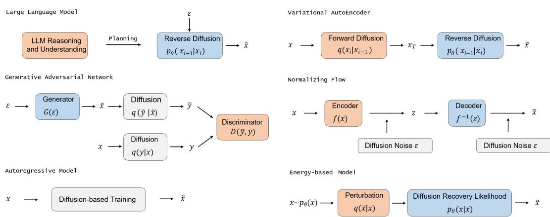
Fig. 3. Illustrations of works incorporating diffusion models with other generative models, such as : LLM [347] where a diffusion model is guided by the LLM planning, VAE [255] where a diffusion model is applied on a latent space, GAN [311] where noise is injected to the discriminator input, normalizing flow [370] where noise is injected in both forward and backward processes in the flow, autoregressive model [116] where the training objective is similar to diffusion models, and EBM [83] where a sequence of EBMs is learned by diffusion recovery likelihood.

In a continuous-time setting, Song et al. (2021) [285], Huang et al. (2021) [119], and Kingma et al. (2021) [154] demonstrate that the score matching objective may be approximated by the Evidence Lower Bound (ELBO) of a deep hierarchical VAE. Consequently, optimizing a diffusion model can be seen as training an infinitely deep hierarchical VAE—a finding that supports the common belief that Score SDE diffusion models can be interpreted as the continuous limit of hierarchical VAEs.

The Latent Score-Based Generative Model (LSGM) [299] furthers this line of research by illustrating that the ELBO can be considered a specialized score matching objective in the context of latent space diffusion. Though the crossentropy term in the ELBO is intractable, it can be transformed into a tractable score matching objective by viewing the score-based generative model as an infinitely deep VAE.

#### 6.3 Generative Adversarial Networks and Connections with Diffusion Models

Generative Adversarial Networks (GANs) [51, 88, 100] mainly consist of two models: a generator and a discriminator . These two models are typically constructed by neural networks but could be implemented in any form of a differentiable system that maps input data from one space to another. The optimization of GANs can be viewed as a mini-max optimization problem with value function (, ):

$$\min\max_{G}\mathbb{E}_{\mathbf{x}\sim p_{data}(\mathbf{x})}\left[\log D(\mathbf{x})\right]+\mathbb{E}_{\mathbf{z}\sim p_{\mathbf{z}}(\mathbf{z})}\left[\log(1-D(G(\mathbf{z})))\right].\tag{42}$$

The generator aims to generate new examples and implicitly model the data distribution. The discriminator is usually a binary classifier that is used to identify generated examples from true examples with maximally possible accuracy. The optimization process ends at a saddle point that produces a minimum about the generator and a maximum about the discriminator. Namely, the goal of GAN optimization is to achieve Nash equilibrium [250]. At that point, the generator can be considered that it has captured the accurate distribution of real examples.

One of the issues of GAN is the instability in the training process, which is mainly caused by the non-overlapping between the distribution of input data and that of the generated data. One solution is to inject noise into the discriminator input for widening the support of both the generator and discriminator distributions. Taking advantage of the flexible diffusion model, Wang et al. (2022) [311] inject noise to the discriminator with an adaptive noise schedule determined by a diffusion model. On the other hand, GAN can facilitate sampling speed of diffusion models. Xiao et al. (2021) [324] show that slow sampling is caused by the Gaussian assumption in the denoising step, which is justified only for small step sizes. As such, each denoising step is modeled by a conditional GAN, allowing larger step size. To ensure the diffusion model captures authentic manifold structures in the data distribution, SADM [346] advocates adversarial training of the diffusion generator against a novel structure discriminator in a minimax game, distinguishing real manifold structures from the generated ones.

### 6.4 Normalizing Flows and Connections with Diffusion Models

Normalizing flows [63, 251] are generative models that generate tractable distributions to model high-dimensional data [65, 155]. Normalizing flows can transform simple probability distribution into an extremely complex probability distribution, which can be used in generative models, reinforcement learning, variational inference, and other fields. Existing normalizing flows are constructed based on the change of variable formula [63, 251]. The trajectory in normalizing flows is formulated by a differential equation. In the discrete-time setting, the mapping from data x to latent z in normalizing flows is a composition of a sequence of bijections, taking the form of = ◦ −1 ◦ . . . ◦ 1. The trajectory {x1, x2, . . . x } in normalizing flows satisfies :

$${\bf x}_{i}=F_{i}({\bf x}_{i-1},\theta),\ {\bf x}_{i-1}=F_{i}^{-1}({\bf x}_{i},\theta)\tag{43}$$

for all ≤ .

Similar to the continuous setting, normalizing flows allow for the retrieval of the exact log-likelihood through a change of variable formula. However, the bijection requirement limits the modeling of complex data in both practical and theoretical contexts [50, 317]. Several works attempt to relax this bijection requirement [65, 317]. For example, DiffFlow [370] introduces a generative modeling algorithm that combines the benefits of both flow-based and diffusion models. As a result, DiffFlow produces sharper boundaries than normalizing flow and learns more general distributions with fewer discretization steps compared to diffusion probabilistic models. Implicit Nonlinear Diffusion Model (INDM) [150] optimizes the pre-encoding process of latent diffusion, which first encodes the original data into the latent space using normalizing flow, and then performs diffusion in the latent space. Using a non-linear diffusion process, INDM can effectively improve the likelihood and the sampling speed.

To scale up the training of CNFs, recent works propose efficient simulation-free approaches [2, 179, 183] by parameterizing a vector field which flows from noise samples to data samples. Lipman et al. (2022) [179] propose Flow Matching (FM) to train CNFs based on constructing explicit conditional probability paths between the noise distribution and each data sample. Wang et al. (2024) [307] conduct an in-depth analysis of the essence of rectification in rectified flow [183] and extend it to rectified diffusion. Besides, they identify that it is not straightness but first-order property is the essential training target of rectified diffusion with theoretical derivations. Yang et al. (2024) further propose Consistency Flow Matching [353], a novel FM method that explicitly enforces self-consistency in the velocity field. Consistency Flow Matching [353] directly defines straight flows starting from different times to the same endpoint,

imposing constraints on their velocity values:

$$\begin{split}&\mathcal{L}_{\theta}=E_{t-d}E_{x_{t},x_{t+\Delta t}}||f_{\theta}(t,x_{t})-f_{\theta^{-}}(t+\Delta t,x_{t+\Delta t})||_{2}^{2}+a||v_{\theta}(t,x_{t})-v_{\theta^{-}}(t+\Delta t,x_{t+\Delta t})||_{2^{-}}^{2}\\ &f_{\theta}(t,x_{t})=x_{t}+(1-t)*v_{\theta}(t,x_{t}),\end{split}\tag{44}$$

where U is the uniform distribution on [0, 1 − Δ], is a positive scalar, Δ denotes a time interval which is a small and positive scalar. − denotes the running average of past values of using exponential moving average (EMA), and +Δ follows a pre-defined distribution which can be efficiently sampled, for example, VP-SDE [111] or OT path [179]. In this way, Consistency Flow Matching [353] innovatively bridges consistency models and flow matching models through the novel concept of straight flows characterized by velocity consistency.

### 6.5 Autoregressive Models and Connections with Diffusion Models

Autoregressive Models (ARMs) work by decomposing the joint distribution of data into a product of conditional distributions using the probability chain rule:

$$\log p({\bf x}_{1:T})=\sum_{t=1}^{T}\log p(x_{t}\mid{\bf x}_{<t})\tag{45}$$

where x< is a shorthand for 1, 2, . . . , −1 [17, 163]. Recent advances in deep learning have facilitated significant progress for various data modalities [34, 207, 264], such as images [45, 302], audio [140, 301], and text [18, 27, 95, 203, 211]. Autoregressive models (ARMs) offer generative capabilities through the use of a single neural network. Sampling from these models requires the same number of network calls as the data's dimensionality. While ARMs are effective density estimators, sampling is a continuous, time-consuming process—particularly for high-dimensional data.

The Autoregressive Diffusion Model (ARDM) [116], on the other hand, is capable of generating arbitrary-order data, including order-agnostic autoregressive models and discrete diffusion models as special cases [9, 117, 276]. Instead of using causal masking on representations like ARMs, the ARDM is trained with an effective objective that mirrors that of diffusion probabilistic models. At the testing stage, the ARDM is able to generate data in parallel—enabling its application to a range of arbitrary-generation tasks.

Ment et al.(2021) [208] incorporates randomized smoothing into autoregressive generative modeling, in order to improve the sample quality. The original data distribution is smoothed by convolving it with a smooth distribution, e.g., a Gaussian or Laplacian kernel. The smoothed data distribution is learned by autoregressive model, and then the learned distribution is denoised by either applying gradient-based denoising approach or introducing another conditional autoregressive model. By choosing the level of smoothness appropriately, the proposed method can improve the sample quality of existing autoregressive models while retaining reasonable likelihoods.

On the other hand, Autoregressive conditional score models (AR-CSM) [210] proposes a score matching method to model the conditional distribution of autoregressive model. The score function of conditional distribution, i.e., ∇ log ( | x<), does not need to be normalized and thus one can use more flexible and advanced neural networks in the model. Furthermore, the univariate conditional score function can be efficiently estimated, even though the dimension of original data might be very high. For inference, AR-CSM uses Langevin dynamics that only need the score function to sample from a density.

### 6.6 Energy-based Models and Connections with Diffusion Models

Energy-based Models (EBMs) [36, 59, 70, 77, 81, 82, 90, 93, 94, 153, 162, 165, 213, 218, 238, 253, 325, 378] can be viewed as one generative version of discriminators [94, 130, 164, 168], while can be learned from unlabeled input data. Let x ∼ data (x) denote a training example, and (x) denote a probability density function that aims to approximates data (x). An energy-based model is defined as:

$$p_{\theta}({\bf x})=\frac{1}{Z_{\theta}}\exp(f_{\theta}({\bf x})),\tag{46}$$

where = ∫ exp( (x))x is the partition function, which is analytically intractable for high-dimensional x. For images, (x) is parameterized by a convolutional neural network with a scalar output. Salimans et al. (2021) [261] compare both constrained score models and energy-based models for modeling the score of the data distribution, finding that constrained score models, i.e., energy based models, can perform just as well as unconstrained models when using a comparable model structure.

Although EBMs have a number of desirable properties, two challenges remain for modeling high-dimensional data. First, learning EBMs by maximizing the likelihood requires MCMC method to generate samples from the model, which can be very computationally expensive. Second, as demonstrated in [217], the energy potentials learned with non-convergent MCMC are not stable, in the sense that samples from long-run Markov chains can be significantly different from the observed samples, and thus it is difficult to evaluate the learned energy potentials. In a recent study, Gao et al. (2021) [83] present a diffusion recovery likelihood method to tractably learn samples from a sequence of EBMs in the reverse process of the diffusion model. Each EBM is trained with recovery likelihood, which aims to maximize the conditional probability of the data at a certain noise level, given their noisy versions at a higher noise level. EBMs maximize the recovery likelihood because it is more tractable than marginal likelihood, as sampling from the conditional distributions is much easier than sampling from the marginal distributions.

# 7 APPLICATIONS OF DIFFUSION MODELS

Diffusion models have recently been employed to address a variety of challenging real-world tasks due to their flexibility and strength. We have grouped these applications into six different categories based on the task: computer vision, natural language processing, temporal data modeling, multi-modal learning, robust learning, and interdisciplinary applications. For each category, we provide a brief introduction to the task, followed by a detailed explanation of how diffusion models have been applied to improve performance. Table 3 summarizes the various applications that have made use of diffusion models.

# 7.1 Unconditional and Conditional Diffusion Models

Before we introduce the applications of diffusion models, we illustrate two basic application paradigms of diffusion models, namely unconditional diffusion models and conditional diffusion models. As a generative model, the history of diffusion models is very similar to VAE, GAN, flow models, and other generative models. They all first developed unconditional generation, and then conditional generation followed closely. Unconditional generation is often used to explore the upper limit of the performance of the generative model, while conditional generation is more about application-level content because it can enable us to control the generation results according to our intentions. In addition to promising generation quality and sample diversity, diffusion models are especially superior in their controllability. The main algorithms of unconditional diffusion models have been well discussed in Sections 2 to 5, in next part, we Manuscript submitted to ACM

| Primary | Secondary | Article |
| --- | --- | --- |
| Computer Vision | Super Resolution, Inpainting, Restoration, Translation, and Editing | [171] [259],[255],[189],[257],[236], [112],[16],[225],[49] |
|  |  | [284],[47],[206],[143],[345],[347] |
|  | Semantic Segmentation | [15],[25],[91],[329] |
|  | Video Generation | [107],[114],[355],[369],[273],[110],[318],[237],[295] |
|  | Point Cloud Completion and Generation | [384],[193],[198],[185],[367] |
|  | Generating Data from Diffusion Models | [349],[26],[385] |
| Natural Language Generation | Natural Language Generation | [9],[175],[42],[86],[106],[61] |
| Temporal Data Modeling | Time Series Imputation | [291],[3],[228],[180] |
|  | Time Series Forecasting | [248],[3],[180] |
|  | Waveform Signal Processing | [39],[159] |
| Multi-Modal Learning | Text-to-Image Generation | [10],[243],[258],[215],[98],[256],[146],[334],[368],[345],[351],[347],[376] |
|  | Scene Graph-to-Image Generation | [342] |
|  | Text-to-3D/4D Generation | [331],[178],[234],[365],[350],[366] |
|  | Text-to-Motion Generation | [292, 369],[151] |
|  | Text-to-Video Generation | [273],[110],[318],[237],[108],[351],[295] |
|  | Text-to-Audio Generation | [235],[336],[320], [170],[288],[120],[152] |
| Robust Learning | Robust Learning | [216],[357],[23],[308],[319],[287] |
| Interdisciplinary Applications | Molecular Graph Modeling | [133],[115],[343],[333],[298], [121],[124],[122] |
|  | Material Design | [327],[196] |
|  | Medical Image Reconstruction | [284],[47],[48],[49],[230],[328] |

Table 3. Summary of all the applications utilizing the diffusion models.

mainly discuss how conditional diffusion models are applied to different applications with different forms of conditions, and choose some typical scenarios for demonstrations.

7.1.1 Conditioning Mechanisms in Diffusion Models. Utilizing different forms of conditions to guide the generation directions of diffusion models are widely used, such as labels, classifiers, texts, images, semantic maps, graphs and so on. However, some of the conditions are structural and complex, thus the methods to condition on them are deserving discussion. There are mainly four kinds of conditioning mechanisms, including concatenation, gradient-based, cross-attention and adaptive layer normalization (adaLN). The concatenation means diffusion models concatenate informative guidance with intermediate denoised targets in diffusion process, such as label embedding and semantic feature maps. The gradient-based mechanism incorporates task-related gradient into the diffusion sampling process for controllable generation. For example, in image generation, one can train an auxiliary classifier on noisy images, and then use gradients to guide the diffusion sampling process towards an arbitrary class label. The cross-attention performs attentional message passing between the guidance and diffusion targets, which is usually conducted in a layer-wise manner in denoising networks. The adaLN mechanism follows the widespread usage of adaptive normalization layers [231] in GANs [142], Scalable Diffusion Models [229] explores replacing standard layer norm layers in transformer-based diffusion backbones with adaptive layer normalization. Instead of directly learning dimension-wise scale and shift parameters, it regresses them from the sum of the time embedding and conditions.

7.1.2 Diffusion with DPO/RLHF. Building on the success of reinforcement learning from human feedback (RLHF) in Large Language Models (LLMs) [11, 224], numerous methods in diffusion models have attempted to use similar approaches for model alignment [75, 167]. Some methods use a pretrained reward model or train a new one to guide the generation process. For instance, ImageReward [330] manually annotated a large dataset of human-preferred images and trained a reward model to assess the alignment between images and human preferences. Some methods bypass the training of a reward model and directly finetune diffusion models on human preference datasets [339]. Diffusion-DPO [306] reformulates Direct Preference Optimization (DPO) to account for a diffusion model's notion of likelihood, utilizing the evidence lower bound to derive a differentiable objective. Recently, Zhang et al. (2024) propose IterComp [376] to iteratively align the base diffusion model with composition-aware model preferences from the model gallery, consisting of six powerful open-source diffusion models, effectively enhancing the performance of base model on conditional

diffusion generation. As demonstrated in Fig. 4, IterComp [376] outperforms other three types of conditional diffusion methods while achieving the best inference efficiency.

![](_page_25_Figure_2.jpeg)

In the heart of an enchanted forest, a majestic tree stands illuminated by glowing mushrooms and tiny lights. Its thick roots form a staircase leading to a cozy door, suggesting a hidden world within. The scene is vibrant and magical, inviting wonder and exploration in this mystical woodland realm.

Fig. 4. Qualitative comparison between IterComp [376] and three types of compositional generation methods: text-controlled, LLM-controlled, and layout-controlled approaches. Colored text denotes the advantages of IterComp [376] in generated images.

7.1.3 Condition Diffusion on Labels and Classifiers. Conditioning diffusion process on the guidance of labels is a straight way to add desired properties into generated samples. However, when labels are limited, it is difficult to enable diffusion models to sufficiently capture the whole distribution of data. SGGM [352] proposes a self-guided diffusion process conditioning on the self-produced hierarchical label set, while You et al. (2023) [359] demonstrate large-scale diffusion models and semi-supervised learners benefit mutually with a few labels via dual pseudo training. Dhariwal and Nichol [60] proposes classifier guidance to boost the sample quality of a diffusion model by using an extra trained classifier. Ho and Salimans [113] jointly train a conditional and an unconditional diffusion model, and find that it is possible to combine the resulting conditional and unconditional scores to obtain a trade-off between sample quality and diversity similar to that obtained by using classifier guidance.

7.1.4 Condition Diffusion on Texts, Images, and Semantic Maps. Recent researches begin to condition diffusion process on the guidance of more semantics, such as texts, images, and semantic maps, to better express rich semantics in samples. DiffuSeq [86] conditions on texts and proposes a seq-to-seq diffusion framework that helps with four NLP tasks. SDEdit [206] conditions on a styled images to make image-to-image translation, while LDM [255] unifies these semantic conditions with flexible latent diffusion. Kindly note that if conditions and diffusion targets are of different modalities, pre-alignment [243, 342] is a practical way to strengthen the guided diffusion. unCLIP [243] and ConPreDiff [345] leverage CLIP latents in text-to-image generation, which have align the semantics between images and texts. RPG [347] conditions on complementary rectangle and contour regions to enable compositional text-to-image generation and complex text-guided image editing. ContextDiff [351] proposes a universal forward-backward consistent diffusion model for better conditioning on various input modalities.

7.1.5 Condition Diffusion on Graphs. Graph-structured data usually exhibits complex relations between nodes, thus conditioning on graphs are extremely hard for diffusion models. SGDiff [342] proposes the first diffusion model specifically designed for scene graph to image generation with a novel masked contrastive pre-training. Such masked pre-training paradigm is general and can be extended to any cross-modal diffusion architectures for both coarse- and finegrained guidance. Other graph-conditioned diffusion models are mainly studied for graph generation. Graphusion [343] conditions on the latent clusters of graph dataset to generate new 2D graphs that greatly align with data distribution. BindDM [121], IPDiff [124] and IRDiff [122] propose to condition on 3D protein graph to generate 3D molecules with equivariant diffusion.

### 7.2 Computer Vision

7.2.1 Image Super Resolution, Inpainting, Restoration, Translation, and Editing. Generative models have been used to tackle a variety of image restoration tasks including super-resolution, inpainting, and translation [16, 58, 74, 128, 171, 225, 244, 379]. Image super-resolution aims to restore high-resolution images from low-resolution inputs, while image inpainting revolves around reconstructing missing or damaged regions in an image.

Several methods make use of diffusion models for these tasks. For example, Super-Resolution via Repeated Refinement (SR3) [259] uses DDPM to enable conditional image generation. SR3 conducts super-resolution through a stochastic, iterative denoising process. The Cascaded Diffusion Model (CDM) [112] consists of multiple diffusion models in sequence, each generating images of increasing resolution. Both the SR3 and CDM directly apply the diffusion process to input images, which leads to larger evaluation steps. In order to allow for the training of diffusion models with limited computational resources, some methods [255, 299] have shifted the diffusion process to the latent space using

![](_page_27_Picture_1.jpeg)

Fig. 5. Image super resolution results produced by LDM [255].

pre-trained autoencoders. The Latent Diffusion Model (LDM) [255] streamlines the training and sampling processes for denoising diffusion models without sacrificing quality.

For inpainting tasks, RePaint [189] features an enhanced denoising strategy that uses resampling iterations to better condition the image. ConPreDiff [345] proposes a universal diffusion model based on context prediction to consistently improve unconditional/conditional image generation and image inpainting (see Figure Fig. 6). Meanwhile, Palette [257] employs conditional diffusion models to create a unified framework for four image generation tasks: colorization, inpainting, uncropping, and JPEG restoration. Image translation focuses on synthesizing images with specific desired

![](_page_27_Picture_5.jpeg)

Fig. 6. Image inpainting results produced by ConPreDiff [345].

styles [128]. SDEdit [206] uses a Stochastic Differential Equation (SDE) prior to improve fidelity. Specifically, it begins Manuscript submitted to ACM

by adding noise to the input image, then denoises the image through the SDE. Denoising Diffusion Restoration Models (DDRM) [143] takes advantage of a pre-trained denoising diffusion generative model for solving linear inverse problem, and demonstrates DDRM's versatility on several image datasets for super-resolution, deblurring, inpainting, and colorization under various amounts of measurement noise. Please refer to Section 7.4.1 for more text-to-image diffusion models.

7.2.2 Semantic Segmentation. Semantic segmentation aims to label each image pixel according to established object categories. Generative pre-training can enhance the label utilization of semantic segmentation models, and recent work has shown that representations learned through DDPM contain high-level semantic information that is useful for segmentation tasks [15, 91]. The few-shot method that leverages these learned representations has outperformed alternatives such as VDVAE [44] and ALAE [232]. Similarly, Decoder Denoising Pretraining (DDeP) [25] integrates diffusion models with denoising autoencoders [305] and delivers promising results on label-efficient semantic segmentation. ODISE [329] explores diffusion models for open-vocabulary segmentation tasks, and proposes a novel implicit captioner to generate captions for images for better utilizing pre-trained large-scale text-to-image diffusion models.

7.2.3 Video Generation. Generating high-quality videos remains a challenge in the deep learning era due to the complexity and spatio-temporal continuity of video frames [341, 362]. Recent research has turned to diffusion models to improve the quality of generated videos [114]. For example, the Flexible Diffusion Model (FDM) [107] uses a generative model to allow for the sampling of any arbitrary subset of video frames, given any other subset. The FDM also includes a specialized architecture designed for this purpose. Additionally, the Residual Video Diffusion (RVD) model [355] utilizes an autoregressive, end-to-end optimized video diffusion model. It generates future frames by amending a deterministic next-frame prediction, using a stochastic residual produced through an inverse diffusion process. Please refer to Section 7.4.5 for more text-to-video diffusion models.

7.2.4 Generating Data from Diffusion Models. Synthesizing datasets from generative models can effectively advance various tasks like classification [12, 309, 385]. Recent works have begun to utilize diffusion models to achieve this goal for vision tasks. For example, Trabucco et al. [297] adopt diffusion models to make effective data augmentation for fewshot image classification. DistDiff [385] proposes a training-free data expansion framework with a distribution-aware diffusion model. It constructs hierarchical prototypes to approximate the real data distribution, and optimizes latent data points in generation process with hierarchical energy guidance. InstructPix2Pix [26] leverages two large pretrained models (i.e., GPT-3 and Stable Diffusion) to generate a large dataset of input-goal-instruction triplet examples, and trains an instruction-following image editing model on the dataset. To enable image editing to reflect chalenging world knowledge and dynamics from both real physical world and virtual media, EditWorld [349], introduces a new task named world-instructed image editing, as the data examples presented in Fig. 7. EditWorld proposes an innovative compositional framework with a set of pretrained LLMs and Diffusion Models, illustrated in Fig. 8, to synthesize a world-instructed training dataset for instruction-following image editing.

7.2.5 Point Cloud Completion and Generation. Point clouds are a critical form of 3D representation for capturing real-world objects. However, scans often generate incomplete point clouds due to partial observation or self-occlusion. Recent studies have applied diffusion models to address this challenge, using them to infer missing parts in order to reconstruct complete shapes. This work has implications for many downstream tasks such as 3D reconstruction, augmented reality, and scene understanding [194, 198, 367].

![](_page_29_Picture_1.jpeg)

**Generated Results** of **InstructPix2Pix Generated Results** of **MagicBrush**

Fig. 7. Comparing EditWorld [349] with InstructPix2Pix and MagicBrush.

![](_page_29_Figure_4.jpeg)

Fig. 8. EditWorld [349] generates a training dataset of world-instructed image editing from two different branches.

Luo et al. 2021 [193] has taken the approach of treating point clouds as particles in a thermodynamic system, using a heat bath to facilitate diffusion from the original distribution to a noise distribution. Meanwhile, the Point-Voxel Diffusion (PVD) model [384] joins denoising diffusion models with the pointvoxel representation of 3D shapes. The Manuscript submitted to ACM

![](_page_30_Figure_1.jpeg)

Fig. 9. The directed graphical model of the diffusion process for point clouds [193].

Point Diffusion-Refinement (PDR) model [198] uses a conditional DDPM to generate a coarse completion from partial observations; it also establishes a point-wise mapping between the generated point cloud and the ground truth.

7.2.6 Anomaly Detection. Anomaly detection is a critical and challenging problem in machine learning [266, 380] and computer vision [337]. Generative models have been shown to own a powerful mechanism for anomaly detection [84, 105, 323], modeling normal or healthy reference data. AnoDDPM [323] utilizes DDPM to corrupt the input image and reconstruct a healthy approximation of the image. These approaches may perform better than alternatives based on adversarial training as they can better model smaller datasets with effective sampling and stable training schemes. DDPM-CD [84] incorporates large numbers of unsupervised remote sensing images into the training process through DDPM. Changes of remote sensed images is detected by utilizing a pre-trained DDPM and applying the multi-scale representations from the diffusion model decoder.

### 7.3 Natural Language Generation

Natural language processing aims to understand, model, and manage human languages from different sources such as text or audio. Text generation has become one of the most critical and challenging tasks in natural language processing [127, 172, 173]. It aims to compose plausible and readable text in the human language given input data (e.g., a sequence and keywords) or random noise. Numerous approaches based on diffusion models have been developed for text generation. Discrete Denoising Diffusion Probabilistic Models (D3PM) [9] introduces diffusion-like generative models for character-level text generation [38]. It generalize the multinomial diffusion model [117] through going beyond corruption processes with uniform transition probabilities. Large autoregressive language models (LMs) is able to generate high-quality text [27, 46, 242, 373]. To reliably deploy these LMs in real-world applications, the text generation process is usually expected to be controllable. It means we need to generate text that can satisfy desired requirements (e.g., topic, syntactic structure). Controlling the behavior of language models without re-training is a major and important problem in text generation [54, 147]. Analog Bits [42] generates the analog bits to represent the discrete variables and further improves the sample quality with self-conditioning and asymmetric time intervals.

Although recent methods have achieved significant successes on controlling simple sentence attributes (e.g., sentiment) [160, 338], there is little progress on complex, fine-grained controls (e.g., syntactic structure). In order to tackle more complex controls, Diffusion-LM [175] proposes a new language model based on continuous diffusion. Diffusion-LM starts with a sequence of Gaussian noise vectors and incrementally denoises them into vectors corresponding to words. The gradual denoising steps help produce hierarchical continuous latent representations. This hierarchical and continuous latent variable can make it possible for simple, gradient-based methods to accomplish complex control. Manuscript submitted to ACM

Similarly, DiffuSeq [86] also conducts diffusion process in latent space and proposes a new conditional diffusion model to accomplish more challenging text-to-text generation tasks. Ssd-LM [106] performs diffusion on the natural vocabulary space instead of a learned latent space, allowing the model to incorporate classifier guidance and modular control without any adaptation of off-the-shelf classifiers. CDCD [61] proposes to model categorical data (including texts) with diffusion models that are continuous both in time and input space, and designs a score interpolation technique for optimization.

# 7.4 Multi-Modal Generation

7.4.1 Text-to-Image Generation. Vision-language models have attracted a lot of attention recently due to the number of potential applications [240]. Text-to-Image generation is the task of generating a corresponding image from a descriptive text [69, 146, 300]. Blended diffusion [10] utilizes both pre-trained DDPM [60] and CLIP [240] models, and it proposes a solution for region-based image editing for general purposes, which uses natural language guidance and is applicable to real and diverse images. On the other hand, unCLIP (DALLE-2) [243] proposes a two-stage approach, a prior model that can generate a CLIP-based image embedding conditioned on a text caption, and a diffusion-based decoder that can generate an image conditioned on the image embedding. Recently, Imagen [258] proposes a text-to-image diffusion model and a comprehensive benchmark for performance evaluation. It shows that Imagen performs well against the state-of-the-art approaches including VQ-GAN+CLIP [52], Latent Diffusion Models [188], and DALL-E 2 [243]. Inspired

![](_page_31_Figure_4.jpeg)

Fig. 10. Synthesis examples demonstrating text-to-image capabilities of for various text prompts with LDM, Imagen, and ContextDiff [351]. Manuscript submitted to ACM

by the ability of guided diffusion models [60, 113] to generate photorealistic samples and the ability of text-to-image models to handle free-form prompts, GLIDE [215] applies guided diffusion to the application of text-conditioned image synthesis. VQ-Diffusion [98] proposes a vector-quantized diffusion model for text-to-image generation, and it eliminates the unidirectional bias and avoids accumulative prediction errors. Versatile Diffusion [334] proposes the first unified multi-flow multimodal diffusion framework, which supports image-to-text, image-variation, text-to-image, and text-variation, and can be further extended to other applications such as semantic-style disentanglement, image-text dual-guided generation, latent image-to-text-to-image editing, and more. Following Versatile Diffusion, UniDiffuser [14] proposes a unified diffusion model framework based on Transformer, which can fit multimodal data distributions and simultaneously handle text-to-image, image-to-text, and joint image-text generation tasks. ConPreDiff [345] for the first time incorporates context prediction into text-to-image diffusion models, and significantly improves generation performance without additional inference costs. ContextDiff [351] proposes general contextualized diffusion model by incorporating the cross-modal context encompassing interactions and alignments into forward and reverse processes. A qualitative comparison between these models are presented in Fig. 10.

![](_page_32_Figure_2.jpeg)

Fig. 11. Overview of RPG [347] framework for text-to-image generation.

A new interesting line of diffusion model research is to leverage the pre-trained text-to-image diffusion model for more complex or fine-grained control of synthesis results. DreamBooth [256] presents the first technique that tackles the new challenging problem of subject-driven generation, allowing users, from just a few casually captured images of a subject, to recontextualize subjects, modify their properties, original art renditions, and more. Different from those image diffusion models conditioned on text prompts, ControlNet [368] attempts to control pre-trained large diffusion models to support additional semantic maps, like edge maps, segmentation maps, keypoints, shape normals, depths, etc. However, most methods often face challenges when handling complex text prompts involving multiple objects with multiple attributes and relationships. To this end, RPG [347] proposes a brand new training-free text-to-image generation/editing framework harnessing the powerful chain-of-thought reasoning ability of multimodal LLMs [377] to enhance the compositionality of text-to-image diffusion models. This new RPG framework unifies both text-guided image generation (in Fig. 11) and image editing (in Fig. 12) tasks in a closed-loop fashion. Notably, as demonstrated in Fig. 13, RPG outperforms all SOTA methods, such as SDXL [233] and DALL-E 3 [20], demonstrate its

![](_page_33_Figure_1.jpeg)

Fig. 12. RPG [347] can unify text-guided image generation and editing in a closed-loop approach.

superiority. Furthermore, RPG framework is user-friendly, and can generalize to different MLLM architectures and diffusion backbones (e.g., ControlNet).

7.4.2 Scene Graph-to-Image Generation. Despite text-to-image generation models has made exciting progress from natural language descriptions, they struggle to faithfully reproduce complex sentences with many objects and relationships. Generating images from scene graphs (SGs) is an important and challenging task for generative models [135]. Traditional methods [109, 135, 176] mainly predict an image-like layout from SGs, then generate images based on the layout. However, such intermediate representations would lose some semantics in SGs, and recent diffusion models [255] are also unable to address this limitation. SGDiff [342] proposes the first diffusion model specifically for image generation from scene graphs (Fig. 14), and learns a continuous SG embedding to condition the latent diffusion model, which has been globally and locally semantically-aligned between SGs and images by the designed masked contrastive pre-training. SGDiff can generate images that better express the intensive and complex relations in SGs compared with both non-diffusion and diffusion methods. However, high-quality paired SG-image datasets are scarce and small-scale, how to leverage large-scale text-image datasets to augment the training or provide a semantic diffusion prior for better initialization is still an open problem.

7.4.3 Text-to-3D Generation. 3D content generation [139, 178, 234, 331] has been in high demand for a wide range of applications, including gaming, entertainment, and robotics simulation. Augmenting 3D content generation with natural language could considerably help with both novices and experienced artists. DreamFusion [234] adopts a pre-trained 2D text-to-image diffusion model to perform text-to-3D synthesis. It optimizes a randomly-initialized 3D model (a Neural Radiance Field, or NeRF) with a probability density distillation loss, which utilizes a 2D diffusion model as a prior for optimization of a parametric image generator. To obtain fast and high-resolution optimization of NeRF, Magic3D [178] proposes a two-stage diffusion framework built on cascaded low-resolution image diffusion prior and high-resolution Manuscript submitted to ACM

![](_page_34_Figure_1.jpeg)

**Prompt:** A beautiful landscape with a river in the middle, the left of the river is in the **evening** and in the **winter** with a big iceberg and a small village while some people are skiing on the river and some people are skating, the right of the river is in the **summer** with a **volcano** in the **morning** and a small village while some people are playing.

![](_page_34_Figure_3.jpeg)

**Left Prompt:** A Chinese general wearing a crown, with whiskers and **golden Chinese** style armor, standing with a **majestic dragon head** on his **chest**, symbolizing his strength, wearing **black** and **gold boots**. His appearance exudes a sense of authority, wisdom, and an unyielding spirit , embodying the ideal ancient Chinese hero.

**Right Prompt**: This painting is a quintessential example of ancient Chinese ink art , At the top of the painting , towering mountains shrouded in **mist rise majestically**. The mountains' craggy peaks are sketched with fine , precise lines , typical of traditional Chinese ink art. A **slender swirling mists**, meandering waterfall begins its descent here , its water appearing almost ethereal amidst the soft. In the middle section, the **waterfall cascades energetically** , creating a dynamic contrast with the serene mountains above. **Lush pine trees** , rendered with graceful , flowing brush strokes , flank the waterfall. These trees appear to dance with the rhythm of the water , adding a vibrant life to the scene. At the bottom , the waterfall concludes its journey in a tranquil pool. The water's surface is calm , reflecting the surrounding nature and the sky above. Here , **delicate flowers** and **small shrubs** are **depicted along** the **water's edge** , symbolizing peace and harmony with nature.

Fig. 13. Compared to previous SOTA models, RPG [347] exhibits a superior ability to express intricate and compositional text prompts within generated images (colored text denotes critical part).

![](_page_35_Figure_1.jpeg)

Fig. 14. SGDiff [342] leverages masked contrastive pre-training for scene graph-based image diffusion generation.

latent diffusion prior. In order to achieve high-fidelity 3D creation, Make-It-3D [290] optimizes a neural radiance field by incorporating constraints from the reference image at the frontal view and diffusion prior at novel views, enhancing the coarse model into textured point clouds and increasing realism with diffusion prior and high-quality textures from the reference image. ProlificDreamer [310] presents Variational Score Distillation (VSD), optimizing a distribution of 3D scenes based on textual prompts as random variables to closely align the distribution of rendered images from all perspectives with a pretrained 2D diffusion model, using KL divergence as the measure. IPDreamer [365] further proposes a novel 3D object synthesis framework that enables users to create controllable and high-quality 3D objects effortlessly. It excels in synthesizing a high-quality 3D object which can greatly align with a provided complex image prompt.

Modeling compositional 3D data distribution is a fundamental and critical task for generative models. Current feed-forward methods [270, 271] are primarily capable of generating single objects and face challenges when creating more complex scenes containing multiple objects due to limited training data. Recently, a series of learnable-layout compositional methods have been proposed [43, 73, 80, 104, 303] . These methods combine multiple object-ad-hoc radiance fields and then optimize the positions of the radiance fields from external feedback. For example, Epstein et al. [73] propose learning a distribution of reasonable layouts based solely on the knowledge from a large pre-trained text-to-image model. Vilesov et al. [303] introduce an optimization method based on Monte-Carlo sampling and physical constraints. However, these forms of layout guidance are relatively coarse and not expressive enough for fine-grained control. Yang et al. (2024) [350] address this problem by incorporating semantic embeddings that ensure view consistency and distinctly differentiate objects into SDS processes (namely SemanticSDS [350]), which are flexible and expressive for optimizing 3D scenes. As shown in Fig. 15, SemanticSDS [350] can achieve superior precision and quality in compositional text-to-3D generation over existing methods. Manuscript submitted to ACM

![](_page_36_Figure_1.jpeg)

A rabbit sits atop a large, expensive watch with many shiny gears, made half of iron and half of gold, ea�ng a birthday cake that is in front of the rabbit

![](_page_36_Figure_3.jpeg)

A mannequin adorned with a dress made of feathers and moss stands at the center, flanked by a vase with a single blue tulip and another with blue roses.

![](_page_36_Figure_5.jpeg)

A car with the front right side made of cheese, the front le� side made of sushi, and the back made of LEGO.

Fig. 15. SemanticSDS [350] achieves superior compositional text-to-3d generation results over state-of-the-art baselines, particularly in generating multiple objects with diverse attibutes.

7.4.4 Text-to-Motion Generation. Human motion generation is a fundamental task in computer animation, with applications covering from gaming to robotics [369]. The generate motion is usually a sequence of human poses Manuscript submitted to ACM

represented by joint rotations and positions. Motion Diffusion Model (MDM) [292] adapts a classifier-free diffusionbased generative model for the human motion generation, which is transformer-based, combining insights from motion generation literature, and regularizes the model with geometric losses on the locations and velocities of the motion. FLAME [151] involves a transformer-based diffusion to better handle motion data, which manages variable-length motions and well attend to free-form text. Notably, it can edit the parts of the motion, both frame-wise and joint-wise, without any fine-tuning.

7.4.5 Text-to-Video Generation. Tremendous recent progress in text-to-image diffusion-based generation motivates the development of text-to-video generation [110, 273, 318]. Make-A-Video [273] proposes to extend a diffusion-based text-to-image model to text-to-video through a spatiotemporally factorized diffusion model. It leverages joint text-image prior to bypass the need for paired text-video data, and further presents super-resolution strategies for high-definition, high frame-rate text-to-video generation. Imagen Video [110] generates high definition videos by designing a cascaded video diffusion models, and transfers some findings that work well in the text-to-image setting to video generation, including frozen T5 text encoder and classifier-free guidance. Tune-A-Video [318] introduces one-shot video tuning for text-to-video generation, which eliminates the burden of training with large-scale video datasets. It employs efficient attention tuning and structural inversion to significantly enhance temporal consistency. Text2Video-Zero [148] achieves zero-shot text-to-video synthesis using a pretrained text-to-image diffusion model, ensuring temporal consistency through motion dynamics in latent codes and cross-frame attention. Its goal is to enable affordable text-guided video generation and editing without additional fine-tuning. FateZero [237] is the first framework for temporal-consistent zero-shot text-to-video editing using pre-trained text-to-image diffusion model. It fuses the attention maps in the DDIM inversion and generation processes to maximally preserve the consistency of motion and structure during editing. ContextDiff [351] incorporates the cross-modal context information about the interactions between text condition and video sample into forward and reverse processes, forming a forward-backward consistent video diffusion model for text-to-video generation.

Most of text-to-video diffusion models are trained on fixed-size video datasets, and thus are often limited to generating a relatively small number of frames, leading to significant degradation in quality when tasked with generating longer videos. Several advancements [108, 295, 388] have sought to overcome this limitation through various strategies. Vlogger [388] employs a masked diffusion model for conditional frame input facilitating longer video generation, and StreamingT2V [108] utilizes a ControlNet-like conditioning mechanism to enable auto-regressive video generation. Recent VideoTetris [295] introduces a Spatio-Temporal Compositional Diffusion method for handling scenes with multiple objects and following progressive complex prompts (i.e., compositional text-to-video generation). Besides, VideoTetris develops a new video data preprocessing method and a consistency regularization method called Reference Frame Attention to improve auto-regressive long video generation through enhanced motion dynamics and prompt semantics. Qualitative comparisons in Fig. 16 show that VideoTetris not only generates superior quality compositional videos, but also produces high-quality long videos that align with compositional prompts while maintaining the best consistency.

7.4.6 Text-to-Audio Generation. Text-to-audio generation is the task to transform normal language texts to voice outputs [170, 320]. Grad-TTS [235] presents a novel text-to-speech model with a score-based decoder and diffusion models. It gradually transforms noise predicted by the encoder and is further aligned with text input by the method of Monotonic Alignment Search [239]. Grad-TTS2 [152] improves Grad-TTS in an adaptive way. Diffsound [336] presents a non-autoregressive decoder based on the discrete diffusion model [9, 275], which predicts all the mel-spectrogram Manuscript submitted to ACM

![](_page_38_Figure_1.jpeg)

Fig. 16. Comparing VideoTetris [295] with open-sourced or commercial T2V models in short and long video generation.

![](_page_39_Figure_1.jpeg)

Fig. 17. Overview of retrieval-augmented diffusion models for time series forecasting (RATD [180]). The historical time series is inputted into the retrieval module to for the corresponding references . After that, is concatenated with the noise as the main input for the model . will be utilized as the guidance for the denoising process.

tokens in every single step, and then refines the predicted tokens in the following steps. EdiTTS [288] leverages the score-based text-to-speech model to refine a mel-spectrogram prior that is coarsely modified. Instead of estimating the gradient of data density, ProDiff [120] parameterizes the denoising diffusion model by directly predicting the clean data.

# 7.5 Temporal Data Modeling

7.5.1 Time Series Imputation. Time series data are widely used with many important real-world applications [72, 223, 341, 374]. Nevertheless, time series usually contain missing values for multiple reasons, caused by mechanical or artificial errors [272, 289, 356]. Recent years, imputation methods have been greatly for both deterministic imputation [32, 37, 197] and probabilistic imputation [78], including diffusion-based approaches. Conditional Score-based Diffusion models for Imputation (CSDI) [291] presents a novel time series imputation method that leverages score-based diffusion models. Specifically, for the purpose of exploiting correlations within temporal data, it adopts the form of self-supervised training to optimize diffusion models. Its application in some real-world datasets reveals its superiority over previous methods. Controlled Stochastic Differential Equation (CSDE) [228] proposes a novel probabilistic framework for modeling stochastic dynamics with a neural-controlled stochastic differential equation. Structured State Space Diffusion (SSSD) [3] integrates conditional diffusion models and structured state-space models [97] to particularly capture long-term dependencies in time series. It performs well in both time series imputation and forecasting tasks.

7.5.2 Time Series Forecasting. Time series forecasting is the task of forecasting or predicting the future value over a period of time. Neural methods have recently become widely-used for solving the prediction problem with univariate point forecasting methods [222] or univariate probabilistic methods [262]. In the multivariate setting, we also have point forecasting methods [174] as well as probabilistic methods, which explicitly model the data distribution using Gaussian copulas [263], GANs [358], or normalizing flows [249]. TimeGrad [248] presents an autoregressive model for forecasting multivariate probabilistic time series, which samples from the data distribution at each time step through estimating its gradient. It utilizes diffusion probabilistic models, which are closely connected with score matching and energy-based methods. Specifically, it learns gradients by optimizing a variational bound on the data likelihood and transforms white noise into a sample of the distribution of interest through a Markov chain using Langevin sampling [280] during inference time. To handle complex time series forecasting, as illustrated in Fig. 17, Liu et al. (2024) for the Manuscript submitted to ACM

first time introduce Retrieval- Augmented Time series Diffusion (RATD) [180], allowing for greater utilization of the dataset and providing meaningful guidance in the denoising process.

7.5.3 Waveform Signal Processing. In electronics, acoustics, and some related fields, the waveform of a signal is denoted by the shape of its graph as a function of time, independent of its time and magnitude scales. WaveGrad [39] introduces a conditional model for waveform generation that estimates gradients of the data density. It receives a Gaussian white noise signal as input and iteratively refines the signal with a gradient-based sampler. WaveGrad naturally trades inference speed for sample quality by adjusting the number of refinement steps, and make a connection between nonautoregressive and autoregressive models with respect to audio quality. DiffWave [159] presents a versatile and effective diffusion probabilistic model for conditional or unconditional waveform generation. The model is non-autoregressive and is efficiently trained by optimizing a variant of variational bound on the data likelihood. Moreover, it produces high-fidelity audio in different waveform generation tasks, such as class-conditional generation and unconditional generation.

# 7.6 Robust Learning

Robust learning is a class of defense methods that help learning networks that are robust to adversarial perturbations or noises [23, 216, 232, 308, 319, 357]. While adversarial training [200] is viewed as a standard defense method against adversarial attacks for image classifiers, adversarial purification has shown significant performances as an alternative defense method [357], which purifies attacked images into clean images with a standalone purification model. Given an adversarial example, DiffPure [216] diffuses it with a small amount of noise following a forward diffusion process and then restores the clean image with a reverse generative process. Adaptive Denoising Purification (ADP) [357] demonstrates that an EBM trained with denoising score matching [304] can effectively purify attacked images within just a few steps. It further proposes an effective randomized purification scheme, injecting random noises into images before purification. Projected Gradient Descent (PGD) [23] presents a novel stochastic diffusion-based pre-processing robustification, which aims to be a model-agnostic adversarial defense and yield a high-quality denoised outcome. In addition, some works propose to apply a guided diffusion process for advanced adversarial purification [308, 319].

# 7.7 Interdisciplinary Applications

7.7.1 Drug Design and Life Science. Graph Neural Networks [102, 322, 344, 383] and corresponding representation learning [103] techniques have achieved great success [21, 293, 321, 332, 340, 387] in many areas, including modeling molecules/proteins in various tasks ranging from property prediction [71, 85] to molecule/protein generation [131, 138, 195, 268], where a molecule is naturally represented by a node-edge graph. On one hand, recent works propose to pre-train GNN/transformer [192, 382] specifically for molecules/proteins with biomedical or physical insights [182, 364], and achieve remarkable results. On the other hand, more works begin to utilize graph-based diffusion models for enhancing molecule or protein generation. Torsional diffusion [133] presents a new diffusion framework that makes operations on the space of torsion angles with a diffusion process on the hyperspace and an extrinsic-to-intrinsic scoring model. GeoDiff [333] demonstrates that Markov chains evolving with equivariant Markov kernels can produce an invariant distribution, and further design blocks for the Markov kernels to preserve the desirable equivariance property. There are also other works incorporate the equivariance property into 3D molecule generation [115] and protein generation [5, 19]. Motivated by the classical force field methods for simulating molecular dynamics, ConfGF [267] directly estimates the gradient fields of the log density of atomic coordinates in molecular conformation generation.

![](_page_41_Figure_1.jpeg)

Fig. 18. IPDiff [124] incorporates protein-ligand interactions into both forward and reverve processes of molecular diffusion models.

Recently, given a target protein, the design of 3D small drug molecules that can closely bind to the target begins to be promoted by diffusion models [99, 122, 124]. IPDiff [124] proposes a novel 3D molecular diffusion model for structure-based drug design (SBDD). As illustrated in Fig. 18, the pocket-ligand interaction is explicitly considered in both forward and reverse processes with the proposed prior-conditioning and prior-shifting mechanisms. Notably, IPDiff beats all previous diffusion-based and autoregressive generation models regarding binding-related metrics and molecular properties. BindDM [121] proposes a hierarchical complex-subcomplex diffusion model for SBDD tasks, which incorporates essential binding-adaptive subcomplex for 3D molecule diffusion generation. IRDiff [124] proposes an interaction-based retrieval-augmented 3D molecular diffusion model named IRDIFF for SBDD tasks. As deonstrated in Fig. 19, this model guides 3D molecular generation using informative external target-aware references, designing two novel augmentation mechanisms, i.e., retrieval augmentation and self augmentation, to incorporate essential protein-molecule binding structures for target-aware molecular generation.

There are also studies that use diffusion models for protein generation, such as DiffAb. DiffAb [196] proposes for the first time a diffusion-based 3D antibody design framework that models both the sequence and structure of the complementarity-determining regions (CDRs) that determine antibody complementarity. Experiments show that DiffAb can be used for various antibody design tasks, such as jointly generating sequence-structure, designing CDRs with fixed frameworks, and optimizing antibodies. SMCDiff [298] proposes to first learn a distribution over diverse and longer protein backbone structures via an E(3)-equivariant graph neural network, and then efficiently samples scaffolds from this distribution given a motif. The generation results demonstrates the designed backbones is well aligned with AlphaFold2-predicted structures.

7.7.2 Material Design. Solid state materials are the critical foundation of numerous key technologies [28]. Crystal Diffusion Variational Autoencoder (CDVAE) [327] incorporates stability as an inductive bias by proposing a noise conditional score network, which simultaneously utilizes permutation, translation, rotation, and periodic invariance Manuscript submitted to ACM

![](_page_42_Figure_1.jpeg)

Fig. 19. IRDiff [122] designs a interaction-based retrieval-augmented generation frameowrk for SBDD.

properties. Luo et al. (2022) [196] model sequences and structures of complementarity-determining regions with equivariant diffusion, and explicitly target specific antigen structures to generate antibodies at atomic resolution.

7.7.3 Medical Image Reconstruction. An inverse problem is to recover an unknown signal from observed measurements, and it is an important problem in medical image reconstruction of Computed Tomography (CT) and Magnetic Resonance Imaging (MRI) [47, 48, 230, 284, 328]. Song et al. (2021) [284] utilize a score-based generative model to reconstruct an image consistent with both the prior and the observed measurements. Chung et al. (2022) [49] train a continuous time-dependent score function with denoising score matching, and iterate between the numerical SDE solver and data consistency step for reconstruction at the evaluation stage. Peng et al. (2022) [230] perform MR reconstruction by gradually guiding the reverse-diffusion process given observed k-space signal, and propose a coarse-to-fine sampling algorithm for efficient sampling.

# 8 FUTURE DIRECTIONS

Research on diffusion models is in its early stages, with much potential for improvement in both theoretical and empirical aspects. As discussed in early sections, key research directions include efficient sampling and improved likelihood, as well as exploring how diffusion models can handle special data structures, interface with other types of generative models, and be tailored to a range of applications. In addition, we foresee that future research on diffusion models will likely expand to the following avenues.

Revisiting Assumptions. Numerous typical assumptions in diffusion models need to be revisited and analyzed. For example, the assumption that the forward process of diffusion models completely erases any information in data and renders it equivalent to a prior distribution may not always hold. In reality, complete removal of information is unachievable in finite time. It is of great interest to understand when to halt the forward noising process in order to strike a balance between sampling efficiency and sample quality [79]. Recent advances in Schrödinger bridges

and optimal transport [41, 55, 57, 269, 278] provide promising alternative solutions, suggesting new formulations for diffusion models that are capable of converging to a specified prior distribution in finite time.

Theoretical Understanding. Diffusion models have emerged as a powerful framework, notably as the only one that can rival generative adversarial networks (GANs) in most applications without resorting to adversarial training. Key to harnessing this potential is an understanding of why and when diffusion models are effective over alternatives for specific tasks. It is important to identify which fundamental characteristics differentiate diffusion models from other types of generative models, such as variational autoencoders, energy-based models, or autoregressive models. Understanding these distinctions will help elucidate why diffusion models are capable of generating samples of excellent quality while achieving top likelihood. Equally important is the need to develop theoretical guidance for selecting and determining various hyperparameters of diffusion models systematically.

Latent Representations. Unlike variational autoencoders or generative adversarial networks, diffusion models are less effective for providing good representations of data in their latent space. As a result, they cannot be easily used for tasks such as manipulating data based on semantic representations. Furthermore, since the latent space in diffusion models often possesses the same dimensionality as the data space, sampling efficiency is negatively affected and the models may not learn the representation schemes well [132].

AIGC and Diffusion Foundation Models. From Stable Diffusion to ChatGPT, Artificial Intelligence Generated Content (AIGC) has gained much attention in both academic and industrial circles. Generative Pre-Training is the core technique in GPT-1/2/3/4 [220, 224, 241, 242] and (Visual) ChatGPT [316], which exhibits promising generation performance and surprising emergent abilities [314] equipped with Large Language Models (LLMs) [296] and Visual Foundation Models [24, 360, 363]. It is interesting to transfer the generative pre-training (decoder-only) from GPT series to diffusion model class, evaluate the diffusion-based generation performance at scale, and analyse the emergent abilities of diffusion foundation models. Furthermore, combining LLMs with diffusion models have been proved to be a new promising direction [347, 349].

# 9 CONCLUSION

We have provided a comprehensive look at diffusion models from various angles. We began with a self-contained introduction to three fundamental formulations: DDPMs, SGMs, and Score SDEs. We then discussed recent efforts to improve diffusion models, highlighting three major directions: sampling efficiency, likelihood maximization, and new techniques for data with special structures. We also explored connections between diffusion models and other generative models and outlined potential benefits of combining the two. A survey of applications across six domains illustrated the wide-ranging potential of diffusion models. Finally, we outlined possible avenues for future research.

#### REFERENCES

- [1] Josh Achiam, Steven Adler, Sandhini Agarwal, Lama Ahmad, Ilge Akkaya, Florencia Leoni Aleman, Diogo Almeida, Janko Altenschmidt, Sam Altman, Shyamal Anadkat, et al. 2023. Gpt-4 technical report. arXiv preprint arXiv:2303.08774 (2023).
- [2] Michael Samuel Albergo and Eric Vanden-Eijnden. 2022. Building Normalizing Flows with Stochastic Interpolants. In The Eleventh International Conference on Learning Representations.
- [3] Juan Miguel Lopez Alcaraz and Nils Strodthoff. 2022. Diffusion-based Time Series Imputation and Forecasting with Structured State Space Models. arXiv preprint arXiv:2208.09399 (2022).
- [4] Tomer Amit, Eliya Nachmani, Tal Shaharbany, and Lior Wolf. 2021. Segdiff: Image segmentation with diffusion probabilistic models. arXiv preprint arXiv:2112.00390 (2021).

- [5] Namrata Anand and Tudor Achim. 2022. Protein Structure and Sequence Generation with Equivariant Denoising Diffusion Probabilistic Models. arXiv preprint arXiv:2205.15019 (2022).
- [6] Brian DO Anderson. 1982. Reverse-time diffusion equation models. Stochastic Processes and their Applications 12, 3 (1982), 313–326.
- [7] Rohan Anil, Andrew M Dai, Orhan Firat, Melvin Johnson, Dmitry Lepikhin, Alexandre Passos, Siamak Shakeri, Emanuel Taropa, Paige Bailey, Zhifeng Chen, et al. 2023. Palm 2 technical report. arXiv preprint arXiv:2305.10403 (2023).
- [8] Uri M Ascher and Linda R Petzold. 1998. Computer methods for ordinary differential equations and differential-algebraic equations. Vol. 61. Siam.
- [9] Jacob Austin, Daniel D Johnson, Jonathan Ho, Daniel Tarlow, and Rianne van den Berg. 2021. Structured denoising diffusion models in discrete state-spaces. In Advances in Neural Information Processing Systems.
- [10] Omri Avrahami, Dani Lischinski, and Ohad Fried. 2022. Blended diffusion for text-driven editing of natural images. In IEEE Conference on Computer Vision and Pattern Recognition. 18208–18218.
- [11] Yuntao Bai, Andy Jones, Kamal Ndousse, Amanda Askell, Anna Chen, Nova DasSarma, Dawn Drain, Stanislav Fort, Deep Ganguli, Tom Henighan, et al. 2022. Training a helpful and harmless assistant with reinforcement learning from human feedback. arXiv preprint arXiv:2204.05862 (2022).
- [12] Hritik Bansal and Aditya Grover. 2023. Leaving Reality to Imagination: Robust Classification via Generated Datasets. In International Conference on Learning Representations.
- [13] Fan Bao, Chongxuan Li, Jun Zhu, and Bo Zhang. 2021. Analytic-DPM: an Analytic Estimate of the Optimal Reverse Variance in Diffusion Probabilistic Models. In International Conference on Learning Representations.
- [14] Fan Bao, Shen Nie, Kaiwen Xue, Chongxuan Li, Shi Pu, Yaole Wang, Gang Yue, Yue Cao, Hang Su, and Jun Zhu. 2023. One Transformer Fits All Distributions in Multi-Modal Diffusion at Scale. arXiv preprint arXiv:2303.06555 (2023).
- [15] Dmitry Baranchuk, Andrey Voynov, Ivan Rubachev, Valentin Khrulkov, and Artem Babenko. 2021. Label-Efficient Semantic Segmentation with Diffusion Models. In International Conference on Learning Representations.
- [16] Georgios Batzolis, Jan Stanczuk, Carola-Bibiane Schönlieb, and Christian Etmann. 2021. Conditional image generation with score-based diffusion models. arXiv preprint arXiv:2111.13606 (2021).
- [17] Samy Bengio and Yoshua Bengio. 2000. Taking on the curse of dimensionality in joint distributions using neural networks. IEEE Trans. Neural Networks Learn. Syst. (2000).
- [18] Yoshua Bengio, Réjean Ducharme, Pascal Vincent, and Christian Janvin. 2003. A neural probabilistic language model. The journal of machine learning research 3 (2003), 1137–1155.
- [19] Helen M Berman, John Westbrook, Zukang Feng, Gary Gilliland, Talapady N Bhat, Helge Weissig, Ilya N Shindyalov, and Philip E Bourne. 2000. The protein data bank. Nucleic acids research 28, 1 (2000), 235–242.
- [20] James Betker, Gabriel Goh, Li Jing, Tim Brooks, Jianfeng Wang, Linjie Li, Long Ouyang, Juntang Zhuang, Joyce Lee, Yufei Guo, et al. 2023. Improving image generation with better captions. Computer Science. https://cdn. openai. com/papers/dall-e-3. pdf (2023).
- [21] Piotr Bielak, Tomasz Kajdanowicz, and Nitesh V Chawla. 2021. Graph Barlow Twins: A self-supervised representation learning framework for graphs. arXiv preprint arXiv:2106.02466 (2021).
- [22] Mikołaj Bińkowski, Dougal J. Sutherland, Michael Arbel, and Arthur Gretton. 2018. Demystifying MMD GANs. In International Conference on Learning Representations.
- [23] Tsachi Blau, Roy Ganz, Bahjat Kawar, Alex Bronstein, and Michael Elad. 2022. Threat Model-Agnostic Adversarial Defense using Diffusion Models. arXiv preprint arXiv:2207.08089 (2022).
- [24] Rishi Bommasani, Drew A Hudson, Ehsan Adeli, Russ Altman, Simran Arora, Sydney von Arx, Michael S Bernstein, Jeannette Bohg, Antoine Bosselut, Emma Brunskill, et al. 2021. On the opportunities and risks of foundation models. arXiv preprint arXiv:2108.07258 (2021).
- [25] Emmanuel Asiedu Brempong, Simon Kornblith, Ting Chen, Niki Parmar, Matthias Minderer, and Mohammad Norouzi. 2022. Denoising Pretraining for Semantic Segmentation. In IEEE Conference on Computer Vision and Pattern Recognition. 4175–4186.
- [26] Tim Brooks, Aleksander Holynski, and Alexei A Efros. 2023. Instructpix2pix: Learning to follow image editing instructions. In IEEE Conference on Computer Vision and Pattern Recognition. 18392–18402.
- [27] Tom Brown, Benjamin Mann, Nick Ryder, Melanie Subbiah, Jared D Kaplan, Prafulla Dhariwal, Arvind Neelakantan, Pranav Shyam, Girish Sastry, Amanda Askell, et al. 2020. Language models are few-shot learners. In Advances in Neural Information Processing Systems.
- [28] Keith T Butler, Daniel W Davies, Hugh Cartwright, Olexandr Isayev, and Aron Walsh. 2018. Machine learning for molecular and materials science. Nature 559, 7715 (2018), 547–555.
- [29] Ruojin Cai, Guandao Yang, Hadar Averbuch-Elor, Zekun Hao, Serge Belongie, Noah Snavely, and Bharath Hariharan. 2020. Learning gradient fields for shape generation. In European Conference on Computer Vision. Springer, 364–381.
- [30] Andrew Campbell, Joe Benton, Valentin De Bortoli, Tom Rainforth, George Deligiannidis, and Arnaud Doucet. 2022. A Continuous Time Framework for Discrete Denoising Models. arXiv preprint arXiv:2205.14987 (2022).
- [31] Chentao Cao, Zhuo-Xu Cui, Shaonan Liu, Dong Liang, and Yanjie Zhu. 2022. High-Frequency Space Diffusion Models for Accelerated MRI. arXiv preprint arXiv:2208.05481 (2022).
- [32] Wei Cao, Dong Wang, Jian Li, Hao Zhou, Lei Li, and Yitan Li. 2018. Brits: Bidirectional recurrent imputation for time series. In Advances in Neural Information Processing Systems, Vol. 31.
- [33] Nicholas Carlini, Florian Tramer, Krishnamurthy Dvijotham1, and Kolter J. Zico. 2022. (Certified!!) Adversarial Robustness for Free! arXiv preprint arXiv:2206.10550 (2022).

- [34] Huiwen Chang, Han Zhang, Lu Jiang, Ce Liu, and William T Freeman. 2022. Maskgit: Masked generative image transformer. In IEEE Conference on Computer Vision and Pattern Recognition. 11315–11325.
- [35] Introducing ChatGPT. 2022. Introducing ChatGPT.
- [36] Tong Che, Ruixiang Zhang, Jascha Sohl-Dickstein, Hugo Larochelle, Liam Paull, Yuan Cao, and Yoshua Bengio. 2020. Your GAN is Secretly an Energy-based Model and You Should use Discriminator Driven Latent Sampling. arXiv preprint arXiv:2003.06060 (2020).
- [37] Zhengping Che, Sanjay Purushotham, Kyunghyun Cho, David Sontag, and Yan Liu. 2018. Recurrent neural networks for multivariate time series with missing values. Scientific reports 8, 1 (2018), 1–12.
- [38] Ciprian Chelba, Tomas Mikolov, Mike Schuster, Qi Ge, Thorsten Brants, Phillipp Koehn, and Tony Robinson. 2013. One billion word benchmark for measuring progress in statistical language modeling. arXiv preprint arXiv:1312.3005 (2013).
- [39] Nanxin Chen, Yu Zhang, Heiga Zen, Ron J Weiss, Mohammad Norouzi, and William Chan. 2020. WaveGrad: Estimating gradients for waveform generation. arXiv preprint arXiv:2009.00713 (2020).
- [40] Ricky TQ Chen, Yulia Rubanova, Jesse Bettencourt, and David Duvenaud. 2018. Neural ordinary differential equations. arXiv preprint arXiv:1806.07366 (2018).
- [41] Tianrong Chen, Guan-Horng Liu, and Evangelos Theodorou. 2021. Likelihood Training of Schrödinger Bridge using Forward-Backward SDEs Theory. In International Conference on Learning Representations.
- [42] Ting Chen, Ruixiang Zhang, and Geoffrey Hinton. 2022. Analog Bits: Generating Discrete Data using Diffusion Models with Self-Conditioning. arXiv preprint arXiv:2208.04202 (2022).
- [43] Yongwei Chen, Tengfei Wang, Tong Wu, Xingang Pan, Kui Jia, and Ziwei Liu. 2024. Comboverse: Compositional 3d assets creation using spatially-aware diffusion guidance. arXiv preprint arXiv:2403.12409 (2024).
- [44] Rewon Child. 2020. Very Deep VAEs Generalize Autoregressive Models and Can Outperform Them on Images. In International Conference on Learning Representations.
- [45] Rewon Child, Scott Gray, Alec Radford, and Ilya Sutskever. 2019. Generating Long Sequences with Sparse Transformers. CoRR abs/1904.10509 (2019). arXiv:1904.10509 http://arxiv.org/abs/1904.10509
- [46] Aakanksha Chowdhery, Sharan Narang, Jacob Devlin, Maarten Bosma, Gaurav Mishra, Adam Roberts, Paul Barham, Hyung Won Chung, Charles Sutton, Sebastian Gehrmann, et al. 2022. PaLM: Scaling Language Modeling with Pathways. (2022).
- [47] Hyungjin Chung, Eun Sun Lee, and Jong Chul Ye. 2022. MR Image Denoising and Super-Resolution Using Regularized Reverse Diffusion. arXiv preprint arXiv:2203.12621 (2022).
- [48] Hyungjin Chung, Byeongsu Sim, and Jong Chul Ye. 2022. Come-closer-diffuse-faster: Accelerating conditional diffusion models for inverse problems through stochastic contraction. In IEEE Conference on Computer Vision and Pattern Recognition. 12413–12422.
- [49] Hyungjin Chung and Jong Chul Ye. 2022. Score-based diffusion models for accelerated MRI. Medical Image Analysis (2022), 102479.
- [50] Rob Cornish, Anthony Caterini, George Deligiannidis, and Arnaud Doucet. 2020. Relaxing bijectivity constraints with continuously indexed normalising flows. In International Conference on Machine Learning. 2133–2143.
- [51] Antonia Creswell, Tom White, Vincent Dumoulin, Kai Arulkumaran, Biswa Sengupta, and Anil A Bharath. 2018. Generative adversarial networks: An overview. IEEE signal processing magazine 35, 1 (2018), 53–65.
- [52] Katherine Crowson, Stella Biderman, Daniel Kornis, Dashiell Stander, Eric Hallahan, Louis Castricato, and Edward Raff. 2022. Vqgan-clip: Open domain image generation and editing with natural language guidance. arXiv preprint arXiv:2204.08583 (2022).
- [53] Salman UH Dar, Şaban Öztürk, Yilmaz Korkmaz, Gokberk Elmas, Muzaffer Özbey, Alper Güngör, and Tolga Çukur. 2022. Adaptive Diffusion Priors for Accelerated MRI Reconstruction. arXiv preprint arXiv:2207.05876 (2022).
- [54] Sumanth Dathathri, Andrea Madotto, Janice Lan, Jane Hung, Eric Frank, Piero Molino, Jason Yosinski, and Rosanne Liu. 2019. Plug and Play Language Models: A Simple Approach to Controlled Text Generation. In International Conference on Learning Representations.
- [55] Valentin De Bortoli, Arnaud Doucet, Jeremy Heng, and James Thornton. 2021. Simulating diffusion bridges with score matching. arXiv preprint arXiv:2111.07243 (2021).
- [56] Valentin De Bortoli, Emile Mathieu, Michael Hutchinson, James Thornton, Yee Whye Teh, and Arnaud Doucet. 2022. Riemannian score-based generative modeling. arXiv preprint arXiv:2202.02763 (2022).
- [57] Valentin De Bortoli, James Thornton, Jeremy Heng, and Arnaud Doucet. 2021. Diffusion Schrödinger bridge with applications to score-based generative modeling. In Advances in Neural Information Processing Systems, Vol. 34. 17695–17709.
- [58] Jia Deng, Wei Dong, Richard Socher, Li-Jia Li, Kai Li, and Li Fei-Fei. 2009. Imagenet: A large-scale hierarchical image database. In IEEE Conference on Computer Vision and Pattern Recognition. 248–255.
- [59] Guillaume Desjardins, Yoshua Bengio, and Aaron C Courville. 2011. On tracking the partition function. In Advances in Neural Information Processing Systems. 2501–2509.
- [60] Prafulla Dhariwal and Alexander Nichol. 2021. Diffusion models beat gans on image synthesis. In Advances in Neural Information Processing Systems, Vol. 34. 8780–8794.
- [61] Sander Dieleman, Laurent Sartran, Arman Roshannai, Nikolay Savinov, Yaroslav Ganin, Pierre H Richemond, Arnaud Doucet, Robin Strudel, Chris Dyer, Conor Durkan, et al. 2022. Continuous diffusion for categorical data. arXiv preprint arXiv:2211.15089 (2022).
- [62] Laurent Dinh, David Krueger, and Yoshua Bengio. 2015. Nice: Non-linear independent components estimation. ICLR 2015 Workshop Track (2015).
- [63] Laurent Dinh, Jascha Sohl-Dickstein, and Samy Bengio. 2016. Density estimation using real nvp. arXiv preprint arXiv:1605.08803 (2016). Manuscript submitted to ACM

- [64] Laurent Dinh, Jascha Sohl-Dickstein, and Samy Bengio. 2017. Density estimation using Real NVP. In International Conference on Learning Representations. https://openreview.net/forum?id=HkpbnH9lx
- [65] Laurent Dinh, Jascha Sohl-Dickstein, Hugo Larochelle, and Razvan Pascanu. 2019. A RAD approach to deep mixture models. arXiv preprint arXiv:1903.07714 (2019).
- [66] Tim Dockhorn, Arash Vahdat, and Karsten Kreis. 2021. Score-Based Generative Modeling with Critically-Damped Langevin Diffusion. In International Conference on Learning Representations.
- [67] Tim Dockhorn, Arash Vahdat, and Karsten Kreis. 2022. GENIE: Higher-Order Denoising Diffusion Solvers. Advances in Neural Information Processing Systems (2022).
- [68] Carl Doersch. 2016. Tutorial on variational autoencoders. arXiv preprint arXiv:1606.05908 (2016).
- [69] Yifan Du, Zikang Liu, Junyi Li, and Wayne Xin Zhao. 2022. A survey of vision-language pre-trained models. arXiv preprint arXiv:2202.10936 (2022).
- [70] Yilun Du and Igor Mordatch. 2019. Implicit generation and generalization in energy-based models. arXiv preprint arXiv:1903.08689 (2019).
- [71] David K Duvenaud, Dougal Maclaurin, Jorge Iparraguirre, Rafael Bombarell, Timothy Hirzel, Alán Aspuru-Guzik, and Ryan P Adams. 2015. Convolutional networks on graphs for learning molecular fingerprints. In Advances in Neural Information Processing Systems, Vol. 28.
- [72] Emadeldeen Eldele, Mohamed Ragab, Zhenghua Chen, Min Wu, Chee Keong Kwoh, Xiaoli Li, and Cuntai Guan. 2021. Time-Series Representation Learning via Temporal and Contextual Contrasting. arXiv preprint arXiv:2106.14112 (2021).
- [73] Dave Epstein, Ben Poole, Ben Mildenhall, Alexei A Efros, and Aleksander Holynski. 2024. Disentangled 3D Scene Generation with Layout Learning. In International Conference on Machine Learning.
- [74] Patrick Esser, Robin Rombach, and Bjorn Ommer. 2021. Taming transformers for high-resolution image synthesis. In IEEE Conference on Computer Vision and Pattern Recognition. 12873–12883.
- [75] Ying Fan, Olivia Watkins, Yuqing Du, Hao Liu, Moonkyung Ryu, Craig Boutilier, Pieter Abbeel, Mohammad Ghavamzadeh, Kangwook Lee, and Kimin Lee. 2024. Reinforcement learning for fine-tuning text-to-image diffusion models. Advances in Neural Information Processing Systems 36 (2024).
- [76] Charles Fefferman, Sanjoy Mitter, and Hariharan Narayanan. 2016. Testing the manifold hypothesis. Journal of the American Mathematical Society 29, 4 (2016), 983–1049.
- [77] Chelsea Finn, Paul Christiano, Pieter Abbeel, and Sergey Levine. 2016. A connection between generative adversarial networks, inverse reinforcement learning, and energy-based models. arXiv preprint arXiv:1611.03852 (2016).
- [78] Vincent Fortuin, Dmitry Baranchuk, Gunnar Ratsch, and Stephan Mandt. 2020. Gp-vae: Deep probabilistic time series imputation. In International conference on artificial intelligence and statistics. PMLR, 1651–1661.
- [79] Giulio Franzese, Simone Rossi, Lixuan Yang, Alessandro Finamore, Dario Rossi, Maurizio Filippone, and Pietro Michiardi. 2022. How much is enough? a study on diffusion times in score-based generative models. arXiv preprint arXiv:2206.05173 (2022).
- [80] Gege Gao, Weiyang Liu, Anpei Chen, Andreas Geiger, and Bernhard Schölkopf. 2024. Graphdreamer: Compositional 3d scene synthesis from scene graphs. In Proceedings of the IEEE/CVF Conference on Computer Vision and Pattern Recognition. 21295–21304.
- [81] Ruiqi Gao, Yang Lu, Junpei Zhou, Song-Chun Zhu, and Ying Nian Wu. 2018. Learning generative convnets via multi-grid modeling and sampling. In IEEE Conference on Computer Vision and Pattern Recognition. 9155–9164.
- [82] Ruiqi Gao, Erik Nijkamp, Diederik P Kingma, Zhen Xu, Andrew M Dai, and Ying Nian Wu. 2020. Flow contrastive estimation of energy-based models. In IEEE Conference on Computer Vision and Pattern Recognition. 7518–7528.
- [83] Ruiqi Gao, Yang Song, Ben Poole, Ying Nian Wu, and Diederik P Kingma. 2020. Learning energy-based models by diffusion recovery likelihood. arXiv preprint arXiv:2012.08125 (2020).
- [84] Wele Gedara Chaminda Bandara, Nithin Gopalakrishnan Nair, and Vishal M Patel. 2022. Remote Sensing Change Detection (Segmentation) using Denoising Diffusion Probabilistic Models. arXiv e-prints (2022), arXiv–2206.
- [85] Justin Gilmer, Samuel S Schoenholz, Patrick F Riley, Oriol Vinyals, and George E Dahl. 2017. Neural message passing for quantum chemistry. In International Conference on Machine Learning. 1263–1272.
- [86] Shansan Gong, Mukai Li, Jiangtao Feng, Zhiyong Wu, and Lingpeng Kong. 2023. Sequence to sequence text generation with diffusion models. In International Conference on Learning Representations.
- [87] Wenbo Gong and Yingzhen Li. 2021. Interpreting diffusion score matching using normalizing flow. arXiv preprint arXiv:2107.10072 (2021).
- [88] Ian Goodfellow, Jean Pouget-Abadie, Mehdi Mirza, Bing Xu, David Warde-Farley, Sherjil Ozair, Aaron Courville, and Yoshua Bengio. 2014. Generative adversarial nets. In Advances in Neural Information Processing Systems, Vol. 27. 139–144.
- [89] Marco Gori, Gabriele Monfardini, and Franco Scarselli. 2005. A new model for learning in graph domains. In Proceedings. 2005 IEEE international joint conference on neural networks, Vol. 2. 729–734.
- [90] Anirudh Goyal Alias Parth Goyal, Nan Rosemary Ke, Surya Ganguli, and Yoshua Bengio. 2017. Variational walkback: Learning a transition operator as a stochastic recurrent net. In Advances in Neural Information Processing Systems. 4392–4402.
- [91] Alexandros Graikos, Nikolay Malkin, Nebojsa Jojic, and Dimitris Samaras. 2022. Diffusion models as plug-and-play priors. In Advances in Neural Information Processing Systems.
- [92] Will Grathwohl, Ricky T. Q. Chen, Jesse Bettencourt, and David Duvenaud. 2019. Scalable Reversible Generative Models with Free-form Continuous Dynamics. In International Conference on Learning Representations. https://openreview.net/forum?id=rJxgknCcK7

- [93] Will Grathwohl, Kuan-Chieh Wang, Jörn-Henrik Jacobsen, David Duvenaud, Mohammad Norouzi, and Kevin Swersky. 2019. Your Classifier is Secretly an Energy Based Model and You Should Treat it Like One. arXiv preprint arXiv:1912.03263 (2019).
- [94] Will Grathwohl, Kuan-Chieh Wang, Jorn-Henrik Jacobsen, David Duvenaud, and Richard Zemel. 2020. Cutting out the Middle-Man: Training and Evaluating Energy-Based Models without Sampling. arXiv preprint arXiv:2002.05616 (2020).
- [95] Alex Graves. 2013. Generating Sequences With Recurrent Neural Networks. CoRR abs/1308.0850 (2013). arXiv:1308.0850 http://arxiv.org/abs/1308. 0850
- [96] Ulf Grenander and Michael I Miller. 1994. Representations of knowledge in complex systems. Journal of the Royal Statistical Society: Series B (Methodological) 56, 4 (1994), 549–581.
- [97] Albert Gu, Karan Goel, and Christopher Re. 2021. Efficiently Modeling Long Sequences with Structured State Spaces. In International Conference on Learning Representations.
- [98] Shuyang Gu, Dong Chen, Jianmin Bao, Fang Wen, Bo Zhang, Dongdong Chen, Lu Yuan, and Baining Guo. 2022. Vector quantized diffusion model for text-to-image synthesis. In IEEE Conference on Computer Vision and Pattern Recognition. 10696–10706.
- [99] Jiaqi Guan, Wesley Wei Qian, Xingang Peng, Yufeng Su, Jian Peng, and Jianzhu Ma. 2023. 3D Equivariant Diffusion for Target-Aware Molecule Generation and Affinity Prediction. In International Conference on Learning Representations.
- [100] Jie Gui, Zhenan Sun, Yonggang Wen, Dacheng Tao, and Jieping Ye. 2021. A review on generative adversarial networks: Algorithms, theory, and applications. IEEE Transactions on Knowledge and Data Engineering (2021).
- [101] David Ha and Jürgen Schmidhuber. 2018. World models. arXiv preprint arXiv:1803.10122 (2018).
- [102] William L Hamilton, Rex Ying, and Jure Leskovec. 2017. Inductive representation learning on large graphs. In Proceedings of the 31st International Conference on Neural Information Processing Systems. 1025–1035.
- [103] William L Hamilton, Rex Ying, and Jure Leskovec. 2017. Representation learning on graphs: Methods and applications. arXiv preprint arXiv:1709.05584 (2017).
- [104] Haonan Han, Rui Yang, Huan Liao, Jiankai Xing, Zunnan Xu, Xiaoming Yu, Junwei Zha, Xiu Li, and Wanhua Li. 2024. REPARO: Compositional 3D Assets Generation with Differentiable 3D Layout Alignment. arXiv preprint arXiv:2405.18525 (2024).
- [105] Songqiao Han, Xiyang Hu, Hailiang Huang, Mingqi Jiang, and Yue Zhao. 2022. ADBench: Anomaly Detection Benchmark. arXiv preprint arXiv:2206.09426 (2022).
- [106] Xiaochuang Han, Sachin Kumar, and Yulia Tsvetkov. 2022. Ssd-lm: Semi-autoregressive simplex-based diffusion language model for text generation and modular control. arXiv preprint arXiv:2210.17432 (2022).
- [107] William Harvey, Saeid Naderiparizi, Vaden Masrani, Christian Weilbach, and Frank Wood. 2022. Flexible Diffusion Modeling of Long Videos. arXiv preprint arXiv:2205.11495 (2022).
- [108] Roberto Henschel, Levon Khachatryan, Daniil Hayrapetyan, Hayk Poghosyan, Vahram Tadevosyan, Zhangyang Wang, Shant Navasardyan, and Humphrey Shi. 2024. StreamingT2V: Consistent, Dynamic, and Extendable Long Video Generation from Text. arXiv preprint arXiv:2403.14773 (2024).
- [109] Roei Herzig, Amir Bar, Huijuan Xu, Gal Chechik, Trevor Darrell, and Amir Globerson. 2020. Learning canonical representations for scene graph to image generation. In European Conference on Computer Vision. 210–227.
- [110] Jonathan Ho, William Chan, Chitwan Saharia, Jay Whang, Ruiqi Gao, Alexey Gritsenko, Diederik P Kingma, Ben Poole, Mohammad Norouzi, David J Fleet, et al. 2022. Imagen video: High definition video generation with diffusion models. arXiv preprint arXiv:2210.02303 (2022).
- [111] Jonathan Ho, Ajay Jain, and Pieter Abbeel. 2020. Denoising diffusion probabilistic models. In Advances in Neural Information Processing Systems, Vol. 33. 6840–6851.
- [112] Jonathan Ho, Chitwan Saharia, William Chan, David J Fleet, Mohammad Norouzi, and Tim Salimans. 2022. Cascaded Diffusion Models for High Fidelity Image Generation. J. Mach. Learn. Res. 23 (2022), 47–1.
- [113] Jonathan Ho and Tim Salimans. 2022. Classifier-free diffusion guidance. arXiv preprint arXiv:2207.12598 (2022).
- [114] Jonathan Ho, Tim Salimans, Alexey Gritsenko, William Chan, Mohammad Norouzi, and David J Fleet. 2022. Video diffusion models. arXiv preprint arXiv:2204.03458 (2022).
- [115] Emiel Hoogeboom, Victor Garcia Satorras, Clement Vignac, and Max Welling. 2022. Equivariant Diffusion for Molecule Generation in 3D. arXiv e-prints (2022), arXiv–2203.
- [116] Emiel Hoogeboom, Alexey A Gritsenko, Jasmijn Bastings, Ben Poole, Rianne van den Berg, and Tim Salimans. 2021. Autoregressive Diffusion Models. In International Conference on Learning Representations.
- [117] Emiel Hoogeboom, Didrik Nielsen, Priyank Jaini, Patrick Forré, and Max Welling. 2021. Argmax flows and multinomial diffusion: Learning categorical distributions. In Advances in Neural Information Processing Systems, Vol. 34. 12454–12465.
- [118] Chin-Wei Huang, Milad Aghajohari, A. Bose, P. Panangaden, and Aaron C. Courville. 2022. Riemannian Diffusion Models.

- [119] Chin-Wei Huang, Jae Hyun Lim, and Aaron C Courville. 2021. A variational perspective on diffusion-based generative models and score matching. In Advances in Neural Information Processing Systems, Vol. 34. 22863–22876.
- [120] Rongjie Huang, Zhou Zhao, Huadai Liu, Jinglin Liu, Chenye Cui, and Yi Ren. 2022. ProDiff: Progressive Fast Diffusion Model For High-Quality Text-to-Speech. arXiv preprint arXiv:2207.06389 (2022).
- [121] Zhilin Huang, Ling Yang, Zaixi Zhang, Xiangxin Zhou, Yu Bao, Xiawu Zheng, Yuwei Yang, Yu Wang, and Wenming Yang. 2024. Binding-Adaptive Diffusion Models for Structure-Based Drug Design. In The AAAI Conference on Artificial Intelligence.

- [122] Zhilin Huang, Ling Yang, Xiangxin Zhou, Chujun Qin, Yijie Yu, Xiawu Zheng, Zikun Zhou, Wentao Zhang, Yu Wang, and Wenming Yang. 2024. Interaction-based Retrieval-augmented Diffusion Models for Protein-specific 3D Molecule Generation. In International Conference on Machine Learning.
- [123] Zhilin Huang, Ling Yang, Xiangxin Zhou, Zhilong Zhang, Wentao Zhang, Xiawu Zheng, Jie Chen, Yu Wang, CUI Bin, and Wenming Yang. 2024. Protein-ligand interaction prior for binding-aware 3d molecule diffusion models. In International Conference on Learning Representations.
- [124] Zhilin Huang, Ling Yang, Xiangxin Zhou, Zhilong Zhang, Wentao Zhang, Xiawu Zheng, Jie Chen, Yu Wang, Bin CUI, and Wenming Yang. 2024. Protein-Ligand Interaction Prior for Binding-aware 3D Molecule Diffusion Models. In International Conference on Learning Representations.
- [125] Michael F Hutchinson. 1989. A stochastic estimator of the trace of the influence matrix for Laplacian smoothing splines. Communications in Statistics-Simulation and Computation 18, 3 (1989), 1059–1076.
- [126] Aapo Hyvärinen. 2005. Estimation of Non-Normalized Statistical Models by Score Matching. J. Mach. Learn. Res. 6 (2005), 695–709.
- [127] Touseef Iqbal and Shaima Qureshi. 2020. The survey: Text generation models in deep learning. Journal of King Saud University-Computer and Information Sciences (2020).
- [128] Phillip Isola, Jun-Yan Zhu, Tinghui Zhou, and Alexei A Efros. 2017. Image-to-image translation with conditional adversarial networks. In IEEE Conference on Computer Vision and Pattern Recognition. 1125–1134.
- [129] Albert Q Jiang, Alexandre Sablayrolles, Antoine Roux, Arthur Mensch, Blanche Savary, Chris Bamford, Devendra Singh Chaplot, Diego de las Casas, Emma Bou Hanna, Florian Bressand, et al. 2024. Mixtral of experts. arXiv preprint arXiv:2401.04088 (2024).
- [130] Long Jin, Justin Lazarow, and Zhuowen Tu. 2017. Introspective classification with convolutional nets. In Advances in Neural Information Processing Systems, Vol. 30. 823–833.
- [131] Wengong Jin, Regina Barzilay, and Tommi Jaakkola. 2018. Junction tree variational autoencoder for molecular graph generation. In International Conference on Machine Learning. 2323–2332.
- [132] Bowen Jing, Gabriele Corso, Renato Berlinghieri, and Tommi Jaakkola. 2022. Subspace diffusion generative models. arXiv preprint arXiv:2205.01490 (2022).
- [133] Bowen Jing, Gabriele Corso, Jeffrey Chang, Regina Barzilay, and Tommi Jaakkola. 2022. Torsional Diffusion for Molecular Conformer Generation. arXiv preprint arXiv:2206.01729 (2022).
- [134] Jaehyeong Jo, Seul Lee, and Sung Ju Hwang. 2022. Score-based generative modeling of graphs via the system of stochastic differential equations. In International Conference on Machine Learning. PMLR, 10362–10383.
- [135] Justin Johnson, Agrim Gupta, and Li Fei-Fei. 2018. Image generation from scene graphs. In Proceedings of the IEEE conference on computer vision and pattern recognition. 1219–1228.
- [136] Alexia Jolicoeur-Martineau, Ke Li, Rémi Piché-Taillefer, Tal Kachman, and Ioannis Mitliagkas. 2021. Gotta Go Fast When Generating Data with Score-Based Models. (2021).
- [137] Alexia Jolicoeur-Martineau, Remi Piche-Taillefer, Rémi Tachet des Combes, and Ioannis Mitliagkas. 2021. Adversarial score matching and improved sampling for image generation. ArXiv abs/2009.05475 (2021).
- [138] John Jumper, Richard Evans, Alexander Pritzel, Tim Green, Michael Figurnov, Olaf Ronneberger, Kathryn Tunyasuvunakool, Russ Bates, Augustin Žídek, Anna Potapenko, et al. 2021. Highly accurate protein structure prediction with AlphaFold. Nature 596, 7873 (2021), 583–589.
- [139] Heewoo Jun and Alex Nichol. 2023. Shap-e: Generating conditional 3d implicit functions. arXiv preprint arXiv:2305.02463 (2023).
- [140] Nal Kalchbrenner, Erich Elsen, Karen Simonyan, Seb Noury, Norman Casagrande, Edward Lockhart, Florian Stimberg, Aäron van den Oord, Sander Dieleman, and Koray Kavukcuoglu. 2018. Efficient Neural Audio Synthesis. In International Conference on Machine Learning. 2410–2419.
- [141] Tero Karras, Miika Aittala, Timo Aila, and Samuli Laine. 2022. Elucidating the Design Space of Diffusion-Based Generative Models. arXiv preprint arXiv:2206.00364 (2022).
- [142] Tero Karras, Samuli Laine, and Timo Aila. 2019. A style-based generator architecture for generative adversarial networks. In Proceedings of the IEEE/CVF conference on computer vision and pattern recognition. 4401–4410.
- [143] Bahjat Kawar, Michael Elad, Stefano Ermon, and Jiaming Song. 2022. Denoising diffusion restoration models. arXiv preprint arXiv:2201.11793 (2022).
- [144] Bahjat Kawar, Roy Ganz, and Michael Elad. 2022. Enhancing diffusion-based image synthesis with robust classifier guidance. arXiv preprint arXiv:2208.08664 (2022).
- [145] Bahjat Kawar, Gregory Vaksman, and Michael Elad. 2021. Stochastic image denoising by sampling from the posterior distribution. In Proceedings of the IEEE/CVF International Conference on Computer Vision. 1866–1875.
- [146] Bahjat Kawar, Shiran Zada, Oran Lang, Omer Tov, Huiwen Chang, Tali Dekel, Inbar Mosseri, and Michal Irani. 2022. Imagic: Text-Based Real Image Editing with Diffusion Models. arXiv preprint arXiv:2210.09276 (2022).
- [147] Nitish Shirish Keskar, Bryan McCann, Lav R Varshney, Caiming Xiong, and Richard Socher. 2019. Ctrl: A conditional transformer language model for controllable generation. arXiv preprint arXiv:1909.05858 (2019).
- [148] Levon Khachatryan, Andranik Movsisyan, Vahram Tadevosyan, Roberto Henschel, Zhangyang Wang, Shant Navasardyan, and Humphrey Shi. 2023. Text2video-zero: Text-to-image diffusion models are zero-shot video generators. arXiv preprint arXiv:2303.13439 (2023).
- [149] Boah Kim, Inhwa Han, and Jong Chul Ye. 2021. Diffusemorph: Unsupervised deformable image registration along continuous trajectory using diffusion models. arXiv preprint arXiv:2112.05149 (2021).

- [150] Dongjun Kim, Byeonghu Na, Se Jung Kwon, Dongsoo Lee, Wanmo Kang, and Il-chul Moon. 2022. Maximum Likelihood Training of Implicit Nonlinear Diffusion Model. In Advances in Neural Information Processing Systems.
- [151] Jihoon Kim, Jiseob Kim, and Sungjoon Choi. 2022. Flame: Free-form language-based motion synthesis & editing. arXiv preprint arXiv:2209.00349 (2022).
- [152] Sungwon Kim, Heeseung Kim, and Sungroh Yoon. 2022. Guided-TTS 2: A Diffusion Model for High-quality Adaptive Text-to-Speech with Untranscribed Data. arXiv preprint arXiv:2205.15370 (2022).
- [153] Taesup Kim and Yoshua Bengio. 2016. Deep directed generative models with energy-based probability estimation. arXiv preprint arXiv:1606.03439 (2016).
- [154] Diederik Kingma, Tim Salimans, Ben Poole, and Jonathan Ho. 2021. Variational diffusion models. In Advances in Neural Information Processing Systems, Vol. 34. 21696–21707.
- [155] Diederik P Kingma and Prafulla Dhariwal. 2018. Glow: Generative flow with invertible 1x1 convolutions. arXiv preprint arXiv:1807.03039 (2018).
- [156] Diederik P Kingma and Max Welling. 2013. Auto-encoding variational bayes. arXiv preprint arXiv:1312.6114 (2013).
- [157] Diederik P Kingma, Max Welling, et al. 2019. An introduction to variational autoencoders. Foundations and Trends® in Machine Learning 12, 4 (2019), 307–392.
- [158] Daphne Koller and Nir Friedman. 2009. Probabilistic graphical models: principles and techniques. MIT press.
- [159] Zhifeng Kong, Wei Ping, Jiaji Huang, Kexin Zhao, and Bryan Catanzaro. 2020. Diffwave: A versatile diffusion model for audio synthesis. arXiv preprint arXiv:2009.09761 (2020).
- [160] Ben Krause, Akhilesh Deepak Gotmare, Bryan McCann, Nitish Shirish Keskar, Shafiq Joty, Richard Socher, and Nazneen Fatema Rajani. 2020. Gedi: Generative discriminator guided sequence generation. arXiv preprint arXiv:2009.06367 (2020).
- [161] Alex Krizhevsky. 2009. Learning Multiple Layers of Features from Tiny Images. (2009).
- [162] Rithesh Kumar, Anirudh Goyal, Aaron Courville, and Yoshua Bengio. 2019. Maximum Entropy Generators for Energy-Based Models. arXiv preprint arXiv:1901.08508 (2019).
- [163] Hugo Larochelle and Iain Murray. 2011. The Neural Autoregressive Distribution Estimator. In Proceedings of the Fourteenth International Conference on Artificial Intelligence and Statistics, AISTATS.
- [164] Justin Lazarow, Long Jin, and Zhuowen Tu. 2017. Introspective neural networks for generative modeling. In Proceedings of the IEEE International Conference on Computer Vision. 2774–2783.
- [165] Yann LeCun, Sumit Chopra, Raia Hadsell, Marc'Aurelio Ranzato, and Fujie Huang. 2006. A tutorial on energy-based learning. Predicting structured data 1, 0 (2006).
- [166] Jin Sub Lee and Philip M Kim. 2022. ProteinSGM: Score-based generative modeling for de novo protein design. bioRxiv (2022).
- [167] Kimin Lee, Hao Liu, Moonkyung Ryu, Olivia Watkins, Yuqing Du, Craig Boutilier, Pieter Abbeel, Mohammad Ghavamzadeh, and Shixiang Shane Gu. 2023. Aligning text-to-image models using human feedback. arXiv preprint arXiv:2302.12192 (2023).
- [168] Kwonjoon Lee, Weijian Xu, Fan Fan, and Zhuowen Tu. 2018. Wasserstein introspective neural networks. In IEEE Conference on Computer Vision and Pattern Recognition. 3702–3711.
- [169] Seul Lee, Jaehyeong Jo, and Sung Ju Hwang. 2022. Exploring Chemical Space with Score-based Out-of-distribution Generation. arXiv preprint arXiv:2206.07632 (2022).
- [170] Alon Levkovitch, Eliya Nachmani, and Lior Wolf. 2022. Zero-Shot Voice Conditioning for Denoising Diffusion TTS Models. arXiv preprint arXiv:2206.02246 (2022).
- [171] Haoying Li, Yifan Yang, Meng Chang, Huajun Feng, Zhi hai Xu, Qi Li, and Yue ting Chen. 2022. SRDiff: Single Image Super-Resolution with Diffusion Probabilistic Models. Neurocomputing 479 (2022), 47–59.
- [172] Junyi Li, Tianyi Tang, Gaole He, Jinhao Jiang, Xiaoxuan Hu, Puzhao Xie, Zhipeng Chen, Zhuohao Yu, Wayne Xin Zhao, and Ji-Rong Wen. 2021. Textbox: A unified, modularized, and extensible framework for text generation. arXiv preprint arXiv:2101.02046 (2021).
- [173] Junyi Li, Tianyi Tang, Wayne Xin Zhao, and Ji-Rong Wen. 2021. Pretrained language models for text generation: A survey. arXiv preprint arXiv:2105.10311 (2021).
- [174] Shiyang Li, Xiaoyong Jin, Yao Xuan, Xiyou Zhou, Wenhu Chen, Yu-Xiang Wang, and Xifeng Yan. 2019. Enhancing the locality and breaking the memory bottleneck of transformer on time series forecasting. In Advances in Neural Information Processing Systems, Vol. 32.
- [175] Xiang Lisa Li, John Thickstun, Ishaan Gulrajani, Percy Liang, and Tatsunori B Hashimoto. 2022. Diffusion-LM Improves Controllable Text Generation. arXiv preprint arXiv:2205.14217 (2022).
- [176] Yikang Li, Tao Ma, Yeqi Bai, Nan Duan, Sining Wei, and Xiaogang Wang. 2019. Pastegan: A semi-parametric method to generate image from scene graph. Advances in Neural Information Processing Systems 32 (2019).
- [177] Long Lian, Boyi Li, Adam Yala, and Trevor Darrell. 2023. LLM-grounded Diffusion: Enhancing Prompt Understanding of Text-to-Image Diffusion Models with Large Language Models. arXiv preprint arXiv:2305.13655 (2023).
- [178] Chen-Hsuan Lin, Jun Gao, Luming Tang, Towaki Takikawa, Xiaohui Zeng, Xun Huang, Karsten Kreis, Sanja Fidler, Ming-Yu Liu, and Tsung-Yi Lin. 2022. Magic3D: High-Resolution Text-to-3D Content Creation. arXiv preprint arXiv:2211.10440 (2022).
- [179] Yaron Lipman, Ricky TQ Chen, Heli Ben-Hamu, Maximilian Nickel, and Matthew Le. 2022. Flow Matching for Generative Modeling. In The Eleventh International Conference on Learning Representations.

- [180] Jingwei Liu, Ling Yang, Hongyan Li, and Shenda Hong. 2024. Retrieval-Augmented Diffusion Models for Time Series Forecasting. In Advances in Neural Information Processing Systems.
- [181] Luping Liu, Yi Ren, Zhijie Lin, and Zhou Zhao. 2021. Pseudo Numerical Methods for Diffusion Models on Manifolds. In International Conference on Learning Representations.
- [182] Shengchao Liu, Hongyu Guo, and Jian Tang. 2023. Molecular geometry pretraining with se (3)-invariant denoising distance matching. In International Conference on Learning Representations.
- [183] Xingchao Liu, Chengyue Gong, et al. 2022. Flow Straight and Fast: Learning to Generate and Transfer Data with Rectified Flow. In The Eleventh International Conference on Learning Representations.
- [184] Xingchao Liu, Lemeng Wu, Mao Ye, et al. 2023. Learning Diffusion Bridges on Constrained Domains. In International Conference on Learning Representations.
- [185] Xingchao Liu, Lemeng Wu, Mao Ye, and Qiang Liu. 2022. Let us Build Bridges: Understanding and Extending Diffusion Generative Models. arXiv preprint arXiv:2208.14699 (2022).
- [186] Aaron Lou, Derek Lim, Isay Katsman, Leo Huang, Qingxuan Jiang, Ser Nam Lim, and Christopher M De Sa. 2020. Neural manifold ordinary differential equations. Advances in Neural Information Processing Systems 33 (2020), 17548–17558.
- [187] Cheng Lu, Kaiwen Zheng, Fan Bao, Jianfei Chen, Chongxuan Li, and Jun Zhu. 2022. Maximum Likelihood Training for Score-based Diffusion ODEs by High Order Denoising Score Matching. In International Conference on Machine Learning. 14429–14460.
- [188] Cheng Lu, Yuhao Zhou, Fan Bao, Jianfei Chen, Chongxuan Li, and Jun Zhu. 2022. DPM-Solver: A Fast ODE Solver for Diffusion Probabilistic Model Sampling in Around 10 Steps. arXiv preprint arXiv:2206.00927 (2022).
- [189] Andreas Lugmayr, Martin Danelljan, Andres Romero, Fisher Yu, Radu Timofte, and Luc Van Gool. 2022. Repaint: Inpainting using denoising diffusion probabilistic models. In IEEE Conference on Computer Vision and Pattern Recognition. 11461–11471.
- [190] Eric Luhman and Troy Luhman. 2021. Knowledge distillation in iterative generative models for improved sampling speed. arXiv preprint arXiv:2101.02388 (2021).
- [191] Calvin Luo. 2022. Understanding Diffusion Models: A Unified Perspective. arXiv preprint arXiv:2208.11970 (2022).
- [192] Shengjie Luo, Tianlang Chen, Yixian Xu, Shuxin Zheng, Tie-Yan Liu, Liwei Wang, and Di He. 2023. One transformer can understand both 2d & 3d molecular data. In International Conference on Learning Representations.
- [193] Shitong Luo and Wei Hu. 2021. Diffusion probabilistic models for 3d point cloud generation. In IEEE Conference on Computer Vision and Pattern Recognition. 2837–2845.
- [194] Shitong Luo and Wei Hu. 2021. Score-based point cloud denoising. In Proceedings of the IEEE/CVF International Conference on Computer Vision. 4583–4592.
- [195] Shitong Luo, Chence Shi, Minkai Xu, and Jian Tang. 2021. Predicting molecular conformation via dynamic graph score matching. In Advances in Neural Information Processing Systems, Vol. 34. 19784–19795.
- [196] Shitong Luo, Yufeng Su, Xingang Peng, Sheng Wang, Jian Peng, and Jianzhu Ma. 2022. Antigen-specific antibody design and optimization with diffusion-based generative models. bioRxiv (2022).
- [197] Yonghong Luo, Xiangrui Cai, Ying Zhang, Jun Xu, et al. 2018. Multivariate time series imputation with generative adversarial networks. In Advances in Neural Information Processing Systems, Vol. 31.
- [198] Zhaoyang Lyu, Zhifeng Kong, XU Xudong, Liang Pan, and Dahua Lin. 2021. A Conditional Point Diffusion-Refinement Paradigm for 3D Point Cloud Completion. In International Conference on Learning Representations.
- [199] Zhaoyang Lyu, Xudong Xu, Ceyuan Yang, Dahua Lin, and Bo Dai. 2022. Accelerating Diffusion Models via Early Stop of the Diffusion Process. arXiv preprint arXiv:2205.12524 (2022).
- [200] Aleksander Madry, Aleksandar Makelov, Ludwig Schmidt, Dimitris Tsipras, and Adrian Vladu. 2018. Towards Deep Learning Models Resistant to Adversarial Attacks. In International Conference on Learning Representations.
- [201] Emile Mathieu and Maximilian Nickel. 2020. Riemannian continuous normalizing flows. Advances in Neural Information Processing Systems 33 (2020), 2503–2515.
- [202] Siyuan Mei, Fuxin Fan, and Andreas Maier. 2022. Metal Inpainting in CBCT Projections Using Score-based Generative Model. arXiv preprint arXiv:2209.09733 (2022).
- [203] Gábor Melis, Chris Dyer, and Phil Blunsom. 2018. On the State of the Art of Evaluation in Neural Language Models. In International Conference on Learning Representations. https://openreview.net/forum?id=ByJHuTgA-
- [204] Chenlin Meng, Kristy Choi, Jiaming Song, and Stefano Ermon. 2022. Concrete Score Matching: Generalized Score Matching for Discrete Data. In Advances in Neural Information Processing Systems.
- [205] Chenlin Meng, Ruiqi Gao, Diederik P Kingma, Stefano Ermon, Jonathan Ho, and Tim Salimans. 2022. On Distillation of Guided Diffusion Models. In NeurIPS 2022 Workshop on Score-Based Methods.
- [206] Chenlin Meng, Yutong He, Yang Song, Jiaming Song, Jiajun Wu, Jun-Yan Zhu, and Stefano Ermon. 2021. Sdedit: Guided image synthesis and editing with stochastic differential equations. In International Conference on Learning Representations.
- [207] Chenlin Meng, Jiaming Song, Yang Song, Shengjia Zhao, and Stefano Ermon. 2020. Improved Autoregressive Modeling with Distribution Smoothing. In International Conference on Learning Representations.

- [208] Chenlin Meng, Jiaming Song, Yang Song, Shengjia Zhao, and Stefano Ermon. 2021. Improved Autoregressive Modeling with Distribution Smoothing. In International Conference on Learning Representations.
- [209] Chenlin Meng, Yang Song, Wenzhe Li, and Stefano Ermon. 2021. Estimating high order gradients of the data distribution by denoising. Advances in Neural Information Processing Systems 34 (2021), 25359–25369.
- [210] Chenlin Meng, Lantao Yu, Yang Song, Jiaming Song, and Stefano Ermon. 2020. Autoregressive score matching. Advances in Neural Information Processing Systems 33 (2020), 6673–6683.
- [211] Stephen Merity, Nitish Shirish Keskar, and Richard Socher. 2018. Regularizing and Optimizing LSTM Language Models. In International Conference on Learning Representations. https://openreview.net/forum?id=SyyGPP0TZ
- [212] Nicholas Metropolis and Stanislaw Ulam. 1949. The monte carlo method. Journal of the American statistical association 44, 247 (1949), 335–341.
- [213] Jiquan Ngiam, Zhenghao Chen, Pang W Koh, and Andrew Y Ng. 2011. Learning deep energy models. In International Conference on Machine Learning. 1105–1112.
- [214] Alexander Quinn Nichol and Prafulla Dhariwal. 2021. Improved denoising diffusion probabilistic models. In International Conference on Machine Learning. 8162–8171.
- [215] Alexander Quinn Nichol, Prafulla Dhariwal, Aditya Ramesh, Pranav Shyam, Pamela Mishkin, Bob Mcgrew, Ilya Sutskever, and Mark Chen. 2022. GLIDE: Towards Photorealistic Image Generation and Editing with Text-Guided Diffusion Models. In International Conference on Machine Learning. 16784–16804.
- [216] Weili Nie, Brandon Guo, Yujia Huang, Chaowei Xiao, Arash Vahdat, and Anima Anandkumar. 2022. Diffusion Models for Adversarial Purification. arXiv preprint arXiv:2205.07460 (2022).
- [217] Erik Nijkamp, Mitch Hill, Tian Han, Song-Chun Zhu, and Ying Nian Wu. 2019. On the anatomy of mcmc-based maximum likelihood learning of energy-based models. arXiv preprint arXiv:1903.12370 (2019).
- [218] Erik Nijkamp, Mitch Hill, Song-Chun Zhu, and Ying Nian Wu. 2019. On Learning Non-Convergent Short-Run MCMC Toward Energy-Based Model. arXiv preprint arXiv:1904.09770 (2019).
- [219] Chenhao Niu, Yang Song, Jiaming Song, Shengjia Zhao, Aditya Grover, and Stefano Ermon. 2020. Permutation invariant graph generation via score-based generative modeling. In International Conference on Artificial Intelligence and Statistics. PMLR, 4474–4484.
- [220] OpenAI. 2023. GPT-4 Technical Report. arXiv preprint arXiv:2303.08774 (2023).
- [221] R OpenAI. 2023. Gpt-4 technical report. arxiv 2303.08774. View in Article 2 (2023), 3.
- [222] Boris N Oreshkin, Dmitri Carpov, Nicolas Chapados, and Yoshua Bengio. 2019. N-BEATS: Neural basis expansion analysis for interpretable time series forecasting. In International Conference on Learning Representations.
- [223] Boris N. Oreshkin, Dmitri Carpov, Nicolas Chapados, and Yoshua Bengio. 2020. N-BEATS: Neural basis expansion analysis for interpretable time series forecasting. In International Conference on Learning Representations.
- [224] Long Ouyang, Jeffrey Wu, Xu Jiang, Diogo Almeida, Carroll Wainwright, Pamela Mishkin, Chong Zhang, Sandhini Agarwal, Katarina Slama, Alex Ray, et al. 2022. Training language models to follow instructions with human feedback. Advances in neural information processing systems 35 (2022), 27730–27744.
- [225] Muzaffer Özbey, Salman UH Dar, Hasan A Bedel, Onat Dalmaz, Şaban Özturk, Alper Güngör, and Tolga Çukur. 2022. Unsupervised Medical Image Translation with Adversarial Diffusion Models. arXiv preprint arXiv:2207.08208 (2022).
- [226] George Papamakarios, Eric T Nalisnick, Danilo Jimenez Rezende, Shakir Mohamed, and Balaji Lakshminarayanan. 2021. Normalizing Flows for Probabilistic Modeling and Inference. J. Mach. Learn. Res. 22, 57 (2021), 1–64.
- [227] Giorgio Parisi. 1981. Correlation functions and computer simulations. Nuclear Physics B 180, 3 (1981), 378–384.
- [228] Sung Woo Park, Kyungjae Lee, and Junseok Kwon. 2021. Neural Markov Controlled SDE: Stochastic Optimization for Continuous-Time Data. In International Conference on Learning Representations.
- [229] William Peebles and Saining Xie. 2022. Scalable Diffusion Models with Transformers. arXiv preprint arXiv:2212.09748 (2022).
- [230] Cheng Peng, Pengfei Guo, S Kevin Zhou, Vishal M Patel, and Rama Chellappa. 2022. Towards performant and reliable undersampled MR reconstruction via diffusion model sampling. In International Conference on Medical Image Computing and Computer-Assisted Intervention. Springer, 623–633.
- [231] Ethan Perez, Florian Strub, Harm De Vries, Vincent Dumoulin, and Aaron Courville. 2018. Film: Visual reasoning with a general conditioning layer. In Proceedings of the AAAI Conference on Artificial Intelligence, Vol. 32.
- [232] Stanislav Pidhorskyi, Donald A Adjeroh, and Gianfranco Doretto. 2020. Adversarial latent autoencoders. In IEEE Conference on Computer Vision and Pattern Recognition. 14104–14113.
- [233] Dustin Podell, Zion English, Kyle Lacey, Andreas Blattmann, Tim Dockhorn, Jonas Müller, Joe Penna, and Robin Rombach. 2023. Sdxl: Improving latent diffusion models for high-resolution image synthesis. arXiv preprint arXiv:2307.01952 (2023).
- [234] Ben Poole, Ajay Jain, Jonathan T Barron, and Ben Mildenhall. 2022. Dreamfusion: Text-to-3d using 2d diffusion. arXiv preprint arXiv:2209.14988 (2022).
- [235] Vadim Popov, Ivan Vovk, Vladimir Gogoryan, Tasnima Sadekova, and Mikhail Kudinov. 2021. Grad-tts: A diffusion probabilistic model for text-to-speech. In International Conference on Machine Learning. 8599–8608.
- [236] Konpat Preechakul, Nattanat Chatthee, Suttisak Wizadwongsa, and Supasorn Suwajanakorn. 2022. Diffusion autoencoders: Toward a meaningful and decodable representation. In IEEE Conference on Computer Vision and Pattern Recognition. 10619–10629.

- [237] Chenyang Qi, Xiaodong Cun, Yong Zhang, Chenyang Lei, Xintao Wang, Ying Shan, and Qifeng Chen. 2023. FateZero: Fusing Attentions for Zero-shot Text-based Video Editing. arXiv preprint arXiv:2303.09535 (2023).
- [238] Yixuan Qiu, Lingsong Zhang, and Xiao Wang. 2019. Unbiased Contrastive Divergence Algorithm for Training Energy-Based Latent Variable Models. In International Conference on Learning Representations.
- [239] Lawrence R Rabiner. 1989. A tutorial on hidden Markov models and selected applications in speech recognition. Proc. IEEE 77, 2 (1989), 257–286.
- [240] Alec Radford, Jong Wook Kim, Chris Hallacy, Aditya Ramesh, Gabriel Goh, Sandhini Agarwal, Girish Sastry, Amanda Askell, Pamela Mishkin, Jack Clark, et al. 2021. Learning transferable visual models from natural language supervision. In International Conference on Machine Learning. 8748–8763.
- [241] Alec Radford, Karthik Narasimhan, Tim Salimans, Ilya Sutskever, et al. 2018. Improving language understanding by generative pre-training. (2018).
- [242] Alec Radford, Jeffrey Wu, Rewon Child, David Luan, Dario Amodei, Ilya Sutskever, et al. 2019. Language models are unsupervised multitask learners. OpenAI blog 1, 8 (2019), 9.
- [243] Aditya Ramesh, Prafulla Dhariwal, Alex Nichol, Casey Chu, and Mark Chen. 2022. Hierarchical text-conditional image generation with clip latents. arXiv preprint arXiv:2204.06125 (2022).
- [244] Aditya Ramesh, Mikhail Pavlov, Gabriel Goh, Scott Gray, Chelsea Voss, Alec Radford, Mark Chen, and Ilya Sutskever. 2021. Zero-shot text-to-image generation. In International Conference on Machine Learning. 8821–8831.
- [245] Martin Raphan and Eero P Simoncelli. 2007. Learning to be Bayesian without supervision. In Advances in neural information processing systems. 1145–1152.
- [246] Martin Raphan and Eero P Simoncelli. 2011. Least squares estimation without priors or supervision. Neural computation 23, 2 (2011), 374–420.
- [247] Kashif Rasul, Calvin Seward, Ingmar Schuster, and Roland Vollgraf. 2021. Autoregressive Denoising Diffusion Models for Multivariate Probabilistic Time Series Forecasting. In International Conference on Machine Learning. 8857–8868.
- [248] Kashif Rasul, Calvin Seward, Ingmar Schuster, and Roland Vollgraf. 2021. Autoregressive denoising diffusion models for multivariate probabilistic time series forecasting. In International Conference on Machine Learning. 8857–8868.
- [249] Kashif Rasul, Abdul-Saboor Sheikh, Ingmar Schuster, Urs M Bergmann, and Roland Vollgraf. 2020. Multivariate Probabilistic Time Series Forecasting via Conditioned Normalizing Flows. In International Conference on Learning Representations.
- [250] Lillian J Ratliff, Samuel A Burden, and S Shankar Sastry. 2013. Characterization and computation of local Nash equilibria in continuous games. In 2013 51st Annual Allerton Conference on Communication, Control, and Computing (Allerton). IEEE, 917–924.
- [251] Danilo Rezende and Shakir Mohamed. 2015. Variational inference with normalizing flows. In International Conference on Machine Learning. 1530–1538.
- [252] Danilo Jimenez Rezende, Shakir Mohamed, and Daan Wierstra. 2014. Stochastic backpropagation and approximate inference in deep generative models. In International Conference on Machine Learning. 1278–1286.
- [253] Benjamin Rhodes, Kai Xu, and Michael U Gutmann. 2020. Telescoping Density-Ratio Estimation. In Advances in Neural Information Processing Systems, Vol. 33. 4905–4916.
- [254] Oren Rippel and Ryan Prescott Adams. 2013. High-dimensional probability estimation with deep density models. arXiv preprint arXiv:1302.5125 (2013).
- [255] Robin Rombach, Andreas Blattmann, Dominik Lorenz, Patrick Esser, and Björn Ommer. 2022. High-resolution image synthesis with latent diffusion models. In IEEE Conference on Computer Vision and Pattern Recognition. 10684–10695.
- [256] Nataniel Ruiz, Yuanzhen Li, Varun Jampani, Yael Pritch, Michael Rubinstein, and Kfir Aberman. 2022. DreamBooth: Fine Tuning Text-to-Image Diffusion Models for Subject-Driven Generation. arXiv preprint arXiv:2208.12242 (2022).
- [257] Chitwan Saharia, William Chan, Huiwen Chang, Chris Lee, Jonathan Ho, Tim Salimans, David Fleet, and Mohammad Norouzi. 2022. Palette: Image-to-image diffusion models. In Special Interest Group on Computer Graphics and Interactive Techniques Conference Proceedings. 1–10.
- [258] Chitwan Saharia, William Chan, Saurabh Saxena, Lala Li, Jay Whang, Emily Denton, Seyed Kamyar Seyed Ghasemipour, Burcu Karagol Ayan, S Sara Mahdavi, Rapha Gontijo Lopes, et al. 2022. Photorealistic Text-to-Image Diffusion Models with Deep Language Understanding. arXiv preprint arXiv:2205.11487 (2022).
- [259] Chitwan Saharia, Jonathan Ho, William Chan, Tim Salimans, David J Fleet, and Mohammad Norouzi. 2022. Image super-resolution via iterative refinement. IEEE Transactions on Pattern Analysis and Machine Intelligence (2022).
- [260] Tim Salimans and Jonathan Ho. 2021. Progressive Distillation for Fast Sampling of Diffusion Models. In International Conference on Learning Representations.
- [261] Tim Salimans and Jonathan Ho. 2021. Should EBMs model the energy or the score?. In Energy Based Models Workshop-International Conference on Learning Representations.
- [262] David Salinas, Michael Bohlke-Schneider, Laurent Callot, Roberto Medico, and Jan Gasthaus. 2019. High-dimensional multivariate forecasting with low-rank gaussian copula processes. In Advances in Neural Information Processing Systems, Vol. 32.
- [263] David Salinas, Valentin Flunkert, Jan Gasthaus, and Tim Januschowski. 2020. DeepAR: Probabilistic forecasting with autoregressive recurrent networks. International Journal of Forecasting 36, 3 (2020), 1181–1191.
- [264] Nikolay Savinov, Junyoung Chung, Mikolaj Binkowski, Erich Elsen, and Aaron van den Oord. 2021. Step-unrolled Denoising Autoencoders for Text Generation. In International Conference on Learning Representations.

- [265] Franco Scarselli, Marco Gori, Ah Chung Tsoi, Markus Hagenbuchner, and Gabriele Monfardini. 2008. The graph neural network model. IEEE transactions on neural networks 20, 1 (2008), 61–80.
- [266] Thomas Schlegl, Philipp Seeböck, Sebastian M Waldstein, Ursula Schmidt-Erfurth, and Georg Langs. 2017. Unsupervised anomaly detection with generative adversarial networks to guide marker discovery. In International conference on information processing in medical imaging. Springer, 146–157.
- [267] Chence Shi, Shitong Luo, Minkai Xu, and Jian Tang. 2021. Learning gradient fields for molecular conformation generation. In International
- [268] Chence Shi, Minkai Xu, Zhaocheng Zhu, Weinan Zhang, Ming Zhang, and Jian Tang. 2020. Graphaf: a flow-based autoregressive model for molecular graph generation. arXiv preprint arXiv:2001.09382 (2020).
- [269] Yuyang Shi, Valentin De Bortoli, George Deligiannidis, and Arnaud Doucet. 2022. Conditional simulation using diffusion Schrödinger bridges. arXiv preprint arXiv:2202.13460 (2022).
- [270] Yichun Shi, Peng Wang, Jianglong Ye, Long Mai, Kejie Li, and Xiao Yang. 2024. MVDream: Multi-view Diffusion for 3D Generation. In The Twelfth International Conference on Learning Representations.
- [271] J Ryan Shue, Eric Ryan Chan, Ryan Po, Zachary Ankner, Jiajun Wu, and Gordon Wetzstein. 2023. 3d neural field generation using triplane diffusion.
- [272] Ikaro Silva, George Moody, Daniel J Scott, Leo A Celi, and Roger G Mark. 2012. Predicting in-hospital mortality of icu patients: The physionet/computing in cardiology challenge 2012. In 2012 Computing in Cardiology. IEEE, 245–248.
- [273] Uriel Singer, Adam Polyak, Thomas Hayes, Xi Yin, Jie An, Songyang Zhang, Qiyuan Hu, Harry Yang, Oron Ashual, Oran Gafni, et al. 2022.
- [274] John Skilling. 1989. The eigenvalues of mega-dimensional matrices. In Maximum Entropy and Bayesian Methods. Springer, 455–466.
- [275] Jascha Sohl-Dickstein, Eric Weiss, Niru Maheswaranathan, and Surya Ganguli. 2015. Deep unsupervised learning using nonequilibrium thermodynamics. In International Conference on Machine Learning. 2256–2265.
- [276] Jascha Sohl-Dickstein, Eric A. Weiss, Niru Maheswaranathan, and Surya Ganguli. 2015. Deep Unsupervised Learning using Nonequilibrium Thermodynamics. In International Conference on Machine Learning, Francis R. Bach and David M. Blei (Eds.). 2256–2265.
- [277] Jiaming Song, Chenlin Meng, and Stefano Ermon. 2020. Denoising Diffusion Implicit Models. In International Conference on Learning Representations.
- [278] Ki-Ung Song. 2022. Applying Regularized Schrödinger-Bridge-Based Stochastic Process in Generative Modeling. arXiv preprint arXiv:2208.07131 (2022).
- [279] Yang Song, Conor Durkan, Iain Murray, and Stefano Ermon. 2021. Maximum likelihood training of score-based diffusion models. In Advances in Neural Information Processing Systems, Vol. 34. 1415–1428.
- [280] Yang Song and Stefano Ermon. 2019. Generative modeling by estimating gradients of the data distribution. In Advances in Neural Information Processing Systems, Vol. 32.
- [281] Yang Song and Stefano Ermon. 2020. Improved techniques for training score-based generative models. In Advances in Neural Information Processing Systems, Vol. 33. 12438–12448.
- [282] Yang Song, Sahaj Garg, Jiaxin Shi, and Stefano Ermon. 2019. Sliced Score Matching: A Scalable Approach to Density and Score Estimation. In Proceedings of the Thirty-Fifth Conference on Uncertainty in Artificial Intelligence, UAI 2019, Tel Aviv, Israel, July 22-25, 2019. 204. http: //auai.org/uai2019/proceedings/papers/204.pdf
- [283] Yang Song and Diederik P Kingma. 2021. How to train your energy-based models. arXiv preprint arXiv:2101.03288 (2021).
- [284] Yang Song, Liyue Shen, Lei Xing, and Stefano Ermon. 2021. Solving Inverse Problems in Medical Imaging with Score-Based Generative Models. In International Conference on Learning Representations.
- [285] Yang Song, Jascha Sohl-Dickstein, Diederik P Kingma, Abhishek Kumar, Stefano Ermon, and Ben Poole. 2020. Score-Based Generative Modeling through Stochastic Differential Equations. In International Conference on Learning Representations.
- [286] James C Spall. 2012. Stochastic optimization. In Handbook of computational statistics. Springer, 173–201.
- [287] Jiachen Sun, Weili Nie, Zhiding Yu, Z Morley Mao, and Chaowei Xiao. 2022. PointDP: Diffusion-driven Purification against Adversarial Attacks on 3D Point Cloud Recognition. arXiv preprint arXiv:2208.09801 (2022).
- [288] Jaesung Tae, Hyeongju Kim, and Taesu Kim. 2021. EdiTTS: Score-based Editing for Controllable Text-to-Speech. arXiv preprint arXiv:2110.02584 (2021).
- [289] Huachun Tan, Guangdong Feng, Jianshuai Feng, Wuhong Wang, Yu-Jin Zhang, and Feng Li. 2013. A tensor-based method for missing traffic data completion. Transportation Research Part C: Emerging Technologies 28 (2013), 15–27.
- [290] Junshu Tang, Tengfei Wang, Bo Zhang, Ting Zhang, Ran Yi, Lizhuang Ma, and Dong Chen. 2023. Make-it-3d: High-fidelity 3d creation from a single image with diffusion prior. arXiv preprint arXiv:2303.14184 (2023).
- [291] Yusuke Tashiro, Jiaming Song, Yang Song, and Stefano Ermon. 2021. CSDI: Conditional score-based diffusion models for probabilistic time series imputation. In Advances in Neural Information Processing Systems, Vol. 34. 24804–24816.
- [292] Guy Tevet, Sigal Raab, Brian Gordon, Yonatan Shafir, Daniel Cohen-Or, and Amit H Bermano. 2022. Human motion diffusion model. arXiv preprint arXiv:2209.14916 (2022).
- [293] Shantanu Thakoor, Corentin Tallec, Mohammad Gheshlaghi Azar, Rémi Munos, Petar Veličković, and Michal Valko. 2021. Bootstrapped representation learning on graphs. arXiv preprint arXiv:2102.06514 (2021).
- Conference on Machine Learning. 9558–9568.
- -
- 
- In Proceedings of the IEEE/CVF Conference on Computer Vision and Pattern Recognition. 20875–20886.
- 
- Make-a-video: Text-to-video generation without text-video data. arXiv preprint arXiv:2209.14792 (2022).
- 

- Manuscript submitted to ACM
- [294] Lucas Theis, Aäron van den Oord, and Matthias Bethge. 2015. A note on the evaluation of generative models. arXiv preprint arXiv:1511.01844 (2015).
- [295] Ye Tian, Ling Yang, Haotian Yang, Yuan Gao, Yufan Deng, Jingmin Chen, Xintao Wang, Zhaochen Yu, Xin Tao, Pengfei Wan, Di Zhang, and Bin Cui. 2024. VideoTetris: Towards Compositional Text-to-Video Generation. Advances in Neural Information Processing Systems (2024).
- [296] Hugo Touvron, Thibaut Lavril, Gautier Izacard, Xavier Martinet, Marie-Anne Lachaux, Timothée Lacroix, Baptiste Rozière, Naman Goyal, Eric Hambro, Faisal Azhar, et al. 2023. Llama: Open and efficient foundation language models. arXiv preprint arXiv:2302.13971 (2023).
- [297] Brandon Trabucco, Kyle Doherty, Max Gurinas, and Ruslan Salakhutdinov. 2023. Effective Data Augmentation With Diffusion Models. In International Conference on Learning Representations.
- [298] Brian L Trippe, Jason Yim, Doug Tischer, Tamara Broderick, David Baker, Regina Barzilay, and Tommi Jaakkola. 2023. Diffusion probabilistic modeling of protein backbones in 3D for the motif-scaffolding problem. In International Conference on Learning Representations.
- [299] Arash Vahdat, Karsten Kreis, and Jan Kautz. 2021. Score-based generative modeling in latent space. In Advances in Neural Information Processing Systems, Vol. 34. 11287–11302.
- [300] Dani Valevski, Matan Kalman, Yossi Matias, and Yaniv Leviathan. 2022. UniTune: Text-Driven Image Editing by Fine Tuning an Image Generation Model on a Single Image. arXiv preprint arXiv:2210.09477 (2022).
- [301] Aäron van den Oord, Sander Dieleman, Heiga Zen, Karen Simonyan, Oriol Vinyals, Alex Graves, Nal Kalchbrenner, Andrew W. Senior, and Koray Kavukcuoglu. 2016. WaveNet: A Generative Model for Raw Audio. In The 9th ISCA Speech Synthesis Workshop.
- [302] Aäron van den Oord, Nal Kalchbrenner, and Koray Kavukcuoglu. 2016. Pixel Recurrent Neural Networks. In International Conference on Machine Learning, Maria-Florina Balcan and Kilian Q. Weinberger (Eds.). 1747–1756.
- [303] Alexander Vilesov, Pradyumna Chari, and Achuta Kadambi. 2023. Cg3d: Compositional generation for text-to-3d via gaussian splatting. arXiv preprint arXiv:2311.17907 (2023).
- [304] Pascal Vincent. 2011. A connection between score matching and denoising autoencoders. Neural computation 23, 7 (2011), 1661–1674.
- [305] Pascal Vincent, Hugo Larochelle, Yoshua Bengio, and Pierre-Antoine Manzagol. 2008. Extracting and composing robust features with denoising autoencoders. In International Conference on Machine Learning. 1096–1103.
- [306] Bram Wallace, Meihua Dang, Rafael Rafailov, Linqi Zhou, Aaron Lou, Senthil Purushwalkam, Stefano Ermon, Caiming Xiong, Shafiq Joty, and Nikhil Naik. 2024. Diffusion model alignment using direct preference optimization. In Proceedings of the IEEE/CVF Conference on Computer Vision and Pattern Recognition. 8228–8238.
- [307] Fu-Yun Wang, Ling Yang, Zhaoyang Huang, Mengdi Wang, and Hongsheng Li. 2024. Rectified Diffusion: Straightness Is Not Your Need in Rectified Flow. arXiv preprint arXiv:2410.07303 (2024).
- [308] Jinyi Wang, Zhaoyang Lyu, Dahua Lin, Bo Dai, and Hongfei Fu. 2022. Guided Diffusion Model for Adversarial Purification. arXiv preprint arXiv:2205.14969 (2022).
- [309] Yufei Wang, Jiayi Zheng, Can Xu, Xiubo Geng, Tao Shen, Chongyang Tao, and Daxin Jiang. 2022. KnowDA: All-in-one knowledge mixture model for data augmentation in few-shot nlp. arXiv preprint arXiv:2206.10265 (2022).
- [310] Zhengyi Wang, Cheng Lu, Yikai Wang, Fan Bao, Chongxuan Li, Hang Su, and Jun Zhu. 2023. ProlificDreamer: High-Fidelity and Diverse Text-to-3D Generation with Variational Score Distillation. arXiv preprint arXiv:2305.16213 (2023).
- [311] Zhendong Wang, Huangjie Zheng, Pengcheng He, Weizhu Chen, and Mingyuan Zhou. 2022. Diffusion-GAN: Training GANs with Diffusion. arXiv preprint arXiv:2206.02262 (2022).
- [312] Daniel Watson, William Chan, Jonathan Ho, and Mohammad Norouzi. 2021. Learning fast samplers for diffusion models by differentiating through sample quality. In International Conference on Learning Representations.
- [313] Daniel Watson, Jonathan Ho, Mohammad Norouzi, and William Chan. 2021. Learning to efficiently sample from diffusion probabilistic models. arXiv preprint arXiv:2106.03802 (2021).
- [314] Jason Wei, Yi Tay, Rishi Bommasani, Colin Raffel, Barret Zoph, Sebastian Borgeaud, Dani Yogatama, Maarten Bosma, Denny Zhou, Donald Metzler, et al. 2022. Emergent Abilities of Large Language Models. Transactions on Machine Learning Research (2022).
- [315] Jay Whang, Mauricio Delbracio, Hossein Talebi, Chitwan Saharia, Alexandros G Dimakis, and Peyman Milanfar. 2022. Deblurring via stochastic refinement. In IEEE Conference on Computer Vision and Pattern Recognition. 16293–16303.
- [316] Chenfei Wu, Shengming Yin, Weizhen Qi, Xiaodong Wang, Zecheng Tang, and Nan Duan. 2023. Visual ChatGPT: Talking, Drawing and Editing with Visual Foundation Models. arXiv preprint arXiv:2303.04671 (2023).
- [317] Hao Wu, Jonas Köhler, and Frank Noe. 2020. Stochastic Normalizing Flows. In Advances in Neural Information Processing Systems, Vol. 33. 5933–5944.
- [318] Jay Zhangjie Wu, Yixiao Ge, Xintao Wang, Weixian Lei, Yuchao Gu, Wynne Hsu, Ying Shan, Xiaohu Qie, and Mike Zheng Shou. 2022. Tune-A-Video: One-Shot Tuning of Image Diffusion Models for Text-to-Video Generation. arXiv preprint arXiv:2212.11565 (2022).
- [319] Quanlin Wu, Hang Ye, and Yuntian Gu. 2022. Guided Diffusion Model for Adversarial Purification from Random Noise. arXiv preprint arXiv:2206.10875 (2022).
- [320] Shoule Wu and Ziqiang Shi. 2021. ItôTTS and ItôWave: Linear Stochastic Differential Equation Is All You Need For Audio Generation. arXiv e-prints (2021), arXiv–2105.
- [321] Shiwen Wu, Fei Sun, Wentao Zhang, Xu Xie, and Bin Cui. 2020. Graph neural networks in recommender systems: a survey. ACM Computing Surveys (CSUR) (2020).

- [322] Zonghan Wu, Shirui Pan, Fengwen Chen, Guodong Long, Chengqi Zhang, and S Yu Philip. 2020. A comprehensive survey on graph neural networks. IEEE transactions on neural networks and learning systems 32, 1 (2020), 4–24.
- [323] Julian Wyatt, Adam Leach, Sebastian M Schmon, and Chris G Willcocks. 2022. AnoDDPM: Anomaly Detection With Denoising Diffusion Probabilistic Models Using Simplex Noise. In IEEE Conference on Computer Vision and Pattern Recognition. 650–656.
- [324] Zhisheng Xiao, Karsten Kreis, and Arash Vahdat. 2021. Tackling the generative learning trilemma with denoising diffusion gans. arXiv preprint arXiv:2112.07804 (2021).
- [325] Jianwen Xie, Yang Lu, Song-Chun Zhu, and Yingnian Wu. 2016. A theory of generative convnet. In International Conference on Machine Learning. 2635–2644.
- [326] Pan Xie, Qipeng Zhang, Zexian Li, Hao Tang, Yao Du, and Xiaohui Hu. 2022. Vector Quantized Diffusion Model with CodeUnet for Text-to-Sign Pose Sequences Generation. arXiv preprint arXiv:2208.09141 (2022).
- [327] Tian Xie, Xiang Fu, Octavian-Eugen Ganea, Regina Barzilay, and Tommi S Jaakkola. 2021. Crystal Diffusion Variational Autoencoder for Periodic Material Generation. In International Conference on Learning Representations.
- [328] Yutong Xie and Quanzheng Li. 2022. Measurement-conditioned Denoising Diffusion Probabilistic Model for Under-sampled Medical Image Reconstruction. arXiv preprint arXiv:2203.03623 (2022).
- [329] Jiarui Xu, Sifei Liu, Arash Vahdat, Wonmin Byeon, Xiaolong Wang, and Shalini De Mello. 2023. Open-Vocabulary Panoptic Segmentation with Text-to-Image Diffusion Models. In IEEE Conference on Computer Vision and Pattern Recognition.
- [330] Jiazheng Xu, Xiao Liu, Yuchen Wu, Yuxuan Tong, Qinkai Li, Ming Ding, Jie Tang, and Yuxiao Dong. 2024. Imagereward: Learning and evaluating human preferences for text-to-image generation. Advances in Neural Information Processing Systems 36 (2024).
- [331] Jiale Xu, Xintao Wang, Weihao Cheng, Yan-Pei Cao, Ying Shan, Xiaohu Qie, and Shenghua Gao. 2022. Dream3D: Zero-Shot Text-to-3D Synthesis Using 3D Shape Prior and Text-to-Image Diffusion Models. arXiv preprint arXiv:2212.14704 (2022).
- [332] Minghao Xu, Hang Wang, Bingbing Ni, Hongyu Guo, and Jian Tang. 2021. Self-supervised graph-level representation learning with local and global structure. In International Conference on Machine Learning. 11548–11558.
- [333] Minkai Xu, Lantao Yu, Yang Song, Chence Shi, Stefano Ermon, and Jian Tang. 2021. GeoDiff: A Geometric Diffusion Model for Molecular Conformation Generation. In International Conference on Learning Representations.
- [334] Xingqian Xu, Zhangyang Wang, Eric Zhang, Kai Wang, and Humphrey Shi. 2022. Versatile Diffusion: Text, Images and Variations All in One Diffusion Model. arXiv preprint arXiv:2211.08332 (2022).
- [335] Tijin Yan, Hongwei Zhang, Tong Zhou, Yufeng Zhan, and Yuanqing Xia. 2021. ScoreGrad: Multivariate Probabilistic Time Series Forecasting with Continuous Energy-based Generative Models. arXiv preprint arXiv:2106.10121 (2021).
- [336] Dongchao Yang, Jianwei Yu, Helin Wang, Wen Wang, Chao Weng, Yuexian Zou, and Dong Yu. 2022. Diffsound: Discrete Diffusion Model for Text-to-sound Generation. arXiv preprint arXiv:2207.09983 (2022).
- [337] Jie Yang, Ruijie Xu, Zhiquan Qi, and Yong Shi. 2021. Visual anomaly detection for images: A survey. arXiv preprint arXiv:2109.13157 (2021).
- [338] Kevin Yang and Dan Klein. 2021. FUDGE: Controlled Text Generation With Future Discriminators. (2021).
- [339] Kai Yang, Jian Tao, Jiafei Lyu, Chunjiang Ge, Jiaxin Chen, Weihan Shen, Xiaolong Zhu, and Xiu Li. 2024. Using human feedback to fine-tune diffusion models without any reward model. In Proceedings of the IEEE/CVF Conference on Computer Vision and Pattern Recognition. 8941–8951.
- [340] Ling Yang and Shenda Hong. 2022. Omni-Granular Ego-Semantic Propagation for Self-Supervised Graph Representation Learning. arXiv preprint arXiv:2205.15746 (2022).
- [341] Ling Yang and Shenda Hong. 2022. Unsupervised Time-Series Representation Learning with Iterative Bilinear Temporal-Spectral Fusion. In International Conference on Machine Learning. 25038–25054.
- [342] Ling Yang, Zhilin Huang, Yang Song, Shenda Hong, Guohao Li, Wentao Zhang, Bin Cui, Bernard Ghanem, and Ming-Hsuan Yang. 2022. Diffusion-Based Scene Graph to Image Generation with Masked Contrastive Pre-Training. arXiv preprint arXiv:2211.11138 (2022).
- [343] Ling Yang, Zhilin Huang, Zhilong Zhang, Zhongyi Liu, Shenda Hong, Wentao Zhang, Wenming Yang, Bin Cui, and Luxia Zhang. 2024. Graphusion: Latent Diffusion for Graph Generation. IEEE Transactions on Knowledge and Data Engineering (2024).
- [344] Ling Yang, Liangliang Li, Zilun Zhang, Xinyu Zhou, Erjin Zhou, and Yu Liu. 2020. Dpgn: Distribution propagation graph network for few-shot learning. In IEEE Conference on Computer Vision and Pattern Recognition. 13390–13399.
- [345] Ling Yang, Jingwei Liu, Shenda Hong, Zhilong Zhang, Zhilin Huang, Zheming Cai, Wentao Zhang, and CUI Bin. 2023. Improving Diffusion-Based Image Synthesis with Context Prediction. In Thirty-seventh Conference on Neural Information Processing Systems.
- [346] Ling Yang, Haotian Qian, Zhilong Zhang, Jingwei Liu, and Bin Cui. 2024. Structure-Guided Adversarial Training of Diffusion Models. In IEEE/CVF Conference on Computer Vision and Pattern Recognition.
- [347] Ling Yang, Zhaochen Yu, Chenlin Meng, Minkai Xu, Stefano Ermon, and Bin Cui. 2024. Mastering Text-to-Image Diffusion: Recaptioning, Planning, and Generating with Multimodal LLMs. In International Conference on Machine Learning.
- [348] Ling Yang, Zhaochen Yu, Tianjun Zhang, Shiyi Cao, Minkai Xu, Wentao Zhang, Joseph E Gonzalez, and Bin Cui. 2024. Buffer of Thoughts: Thought-Augmented Reasoning with Large Language Models. arXiv preprint arXiv:2406.04271 (2024).
- [349] Ling Yang, Bohan Zeng, Jiaming Liu, Hong Li, Minghao Xu, Wentao Zhang, and Shuicheng Yan. 2024. EditWorld: Simulating World Dynamics for Instruction-Following Image Editing. arXiv preprint arXiv:2405.14785 (2024).
- [350] Ling Yang, Zixiang Zhang, Junlin Han, Bohan Zeng, Runjia Li, Philip Torr, and Wentao Zhang. 2024. Semantic Score Distillation Sampling for Compositional Text-to-3D Generation. arXiv preprint arXiv:2410.09009 (2024).

- [351] Ling Yang, Zhilong Zhang, Zhaochen Yu, Jingwei Liu, Minkai Xu, Stefano Ermon, and Bin CUI. 2024. Cross-Modal Contextualized Diffusion Models for Text-Guided Visual Generation and Editing. In International Conference on Learning Representations.
- [352] Ling Yang, Zhilong Zhang, Wentao Zhang, and Shenda Hong. 2023. Score-Based Graph Generative Modeling with Self-Guided Latent Diffusion. (2023). https://openreview.net/forum?id=AykEgQNPJEK
- [353] Ling Yang, Zixiang Zhang, Zhilong Zhang, Xingchao Liu, Minkai Xu, Wentao Zhang, Chenlin Meng, Stefano Ermon, and Bin Cui. 2024. Consistency Flow Matching: Defining Straight Flows with Velocity Consistency. arXiv preprint arXiv:2407.02398 (2024).
- [354] Ruihan Yang and Stephan Mandt. 2022. Lossy Image Compression with Conditional Diffusion Models. arXiv preprint arXiv:2209.06950 (2022).
- [355] Ruihan Yang, Prakhar Srivastava, and Stephan Mandt. 2022. Diffusion probabilistic modeling for video generation. arXiv preprint arXiv:2203.09481 (2022).
- [356] Xiuwen Yi, Yu Zheng, Junbo Zhang, and Tianrui Li. 2016. ST-MVL: filling missing values in geo-sensory time series data. In Proceedings of the 25th International Joint Conference on Artificial Intelligence.
- [357] Jongmin Yoon, Sung Ju Hwang, and Juho Lee. 2021. Adversarial purification with score-based generative models. In International Conference on Machine Learning. 12062–12072.
- [358] Jinsung Yoon, Daniel Jarrett, and Mihaela Van der Schaar. 2019. Time-series generative adversarial networks. In Advances in Neural Information Processing Systems, Vol. 32.
- [359] Zebin You, Yong Zhong, Fan Bao, Jiacheng Sun, Chongxuan Li, and Jun Zhu. 2023. Diffusion Models and Semi-Supervised Learners Benefit Mutually with Few Labels. arXiv preprint arXiv:2302.10586 (2023).
- [360] Jiahui Yu, Zirui Wang, Vijay Vasudevan, Legg Yeung, Mojtaba Seyedhosseini, and Yonghui Wu. 2022. Coca: Contrastive captioners are image-text foundation models. arXiv preprint arXiv:2205.01917 (2022).
- [361] Peiyu Yu, Sirui Xie, Xiaojian Ma, Baoxiong Jia, Bo Pang, Ruiqi Gao, Yixin Zhu, Song-Chun Zhu, and Ying Nian Wu. 2022. Latent Diffusion Energy-Based Model for Interpretable Text Modelling. In International Conference on Machine Learning. 25702–25720.
- [362] Sihyun Yu, Jihoon Tack, Sangwoo Mo, Hyunsu Kim, Junho Kim, Jung-Woo Ha, and Jinwoo Shin. 2022. Generating videos with dynamics-aware implicit generative adversarial networks. arXiv preprint arXiv:2202.10571 (2022).
- [363] Lu Yuan, Dongdong Chen, Yi-Ling Chen, Noel Codella, Xiyang Dai, Jianfeng Gao, Houdong Hu, Xuedong Huang, Boxin Li, Chunyuan Li, et al. 2021. Florence: A new foundation model for computer vision. arXiv preprint arXiv:2111.11432 (2021).
- [364] Sheheryar Zaidi, Michael Schaarschmidt, James Martens, Hyunjik Kim, Yee Whye Teh, Alvaro Sanchez-Gonzalez, Peter Battaglia, Razvan Pascanu, and Jonathan Godwin. 2023. Pre-training via denoising for molecular property prediction. In International Conference on Learning Representations.
- [365] Bohan Zeng, Shanglin Li, Yutang Feng, Ling Yang, Hong Li, Sicheng Gao, Jiaming Liu, Conghui He, Wentao Zhang, Jianzhuang Liu, Baochang Zhang, and Shuicheng Yan. 2023. Ipdreamer: Appearance-controllable 3d object generation with image prompts. arXiv preprint arXiv:2310.05375 (2023).
- [366] Bohan Zeng, Ling Yang, Siyu Li, Jiaming Liu, Zixiang Zhang, Juanxi Tian, Kaixin Zhu, Yongzhen Guo, Fu-Yun Wang, Minkai Xu, Stefano Ermon, and Wentao Zhang. 2024. Trans4D: Realistic Geometry-Aware Transition for Compositional Text-to-4D Synthesis. arXiv preprint arXiv:2410.07155 (2024).
- [367] Xiaohui Zeng, Arash Vahdat, Francis Williams, Zan Gojcic, Or Litany, Sanja Fidler, and Karsten Kreis. 2022. LION: Latent Point Diffusion Models for 3D Shape Generation. In Advances in Neural Information Processing Systems.
- [368] Lvmin Zhang and Maneesh Agrawala. 2023. Adding conditional control to text-to-image diffusion models. arXiv preprint arXiv:2302.05543 (2023).
- [369] Mingyuan Zhang, Zhongang Cai, Liang Pan, Fangzhou Hong, Xinying Guo, Lei Yang, and Ziwei Liu. 2022. Motiondiffuse: Text-driven human motion generation with diffusion model. arXiv preprint arXiv:2208.15001 (2022).
- [370] Qinsheng Zhang and Yongxin Chen. 2021. Diffusion Normalizing Flow. In Advances in Neural Information Processing Systems, Vol. 34. 16280–16291.
- [371] Qinsheng Zhang and Yongxin Chen. 2022. Fast Sampling of Diffusion Models with Exponential Integrator. arXiv preprint arXiv:2204.13902 (2022).
- [372] Qinsheng Zhang, Molei Tao, and Yongxin Chen. 2022. gDDIM: Generalized denoising diffusion implicit models. arXiv preprint arXiv:2206.05564 (2022).
- [373] Susan Zhang, Stephen Roller, Naman Goyal, Mikel Artetxe, Moya Chen, Shuohui Chen, Christopher Dewan, Mona Diab, Xian Li, Xi Victoria Lin, et al. 2022. Opt: Open pre-trained transformer language models. arXiv preprint arXiv:2205.01068 (2022).
- [374] Wenrui Zhang, Ling Yang, Shijia Geng, and Shenda Hong. 2022. Cross Reconstruction Transformer for Self-Supervised Time Series Representation Learning. arXiv preprint arXiv:2205.09928 (2022).
- [375] Xinchen Zhang, Ling Yang, Yaqi Cai, Zhaochen Yu, Kaini Wang, Jiake Xie, Ye Tian, Minkai Xu, Yong Tang, Yujiu Yang, and Bin Cui. 2024. RealCompo: Balancing Realism and Compositionality Improves Text-to-Image Diffusion Models. arXiv preprint arXiv:2402.12908 (2024).
- [376] Xinchen Zhang, Ling Yang, Guohao Li, Yaqi Cai, Jiake Xie, Yong Tang, Yujiu Yang, Mengdi Wang, and Bin Cui. 2024. IterComp: Iterative Composition-Aware Feedback Learning from Model Gallery for Text-to-Image Generation. arXiv preprint arXiv:2410.07171 (2024).
- [377] Zhuosheng Zhang, Aston Zhang, Mu Li, Hai Zhao, George Karypis, and Alex Smola. 2023. Multimodal chain-of-thought reasoning in language models. arXiv preprint arXiv:2302.00923 (2023).
- [378] Junbo Zhao, Michael Mathieu, and Yann LeCun. 2016. Energy-based generative adversarial network. arXiv preprint arXiv:1609.03126 (2016).
- [379] Min Zhao, Fan Bao, Chongxuan Li, and Jun Zhu. 2022. Egsde: Unpaired image-to-image translation via energy-guided stochastic differential equations. arXiv preprint arXiv:2207.06635 (2022).

- [380] Yue Zhao, Zain Nasrullah, and Zheng Li. 2019. PyOD: A Python Toolbox for Scalable Outlier Detection. Journal of Machine Learning Research 20 (2019), 1–7.
- [381] Huangjie Zheng, Pengcheng He, Weizhu Chen, and Mingyuan Zhou. 2022. Truncated diffusion probabilistic models. arXiv preprint arXiv:2202.09671 (2022).
- [382] Gengmo Zhou, Zhifeng Gao, Qiankun Ding, Hang Zheng, Hongteng Xu, Zhewei Wei, Linfeng Zhang, and Guolin Ke. 2023. Uni-mol: A universal 3d molecular representation learning framework. In International Conference on Learning Representations.
- [383] Jie Zhou, Ganqu Cui, Shengding Hu, Zhengyan Zhang, Cheng Yang, Zhiyuan Liu, Lifeng Wang, Changcheng Li, and Maosong Sun. 2020. Graph neural networks: A review of methods and applications. AI Open 1 (2020), 57–81.
- [384] Linqi Zhou, Yilun Du, and Jiajun Wu. 2021. 3d shape generation and completion through point-voxel diffusion. In Proceedings of the IEEE/CVF International Conference on Computer Vision. 5826–5835.
- [385] Haowei Zhu, Ling Yang, Jun-Hai Yong, Wentao Zhang, and Bin Wang. 2024. Distribution-Aware Data Expansion with Diffusion Models. arXiv preprint arXiv:2403.06741 (2024).
- [386] Ye Zhu, Yu Wu, Kyle Olszewski, Jian Ren, Sergey Tulyakov, and Yan Yan. 2022. Discrete contrastive diffusion for cross-modal and conditional generation. arXiv preprint arXiv:2206.07771 (2022).
- [387] Yanqiao Zhu, Yichen Xu, Feng Yu, Qiang Liu, Shu Wu, and Liang Wang. 2020. Deep graph contrastive representation learning. arXiv preprint arXiv:2006.04131 (2020).
- [388] Shaobin Zhuang, Kunchang Li, Xinyuan Chen, Yaohui Wang, Ziwei Liu, Yu Qiao, and Yali Wang. 2024. Vlogger: Make Your Dream A Vlog. arXiv preprint arXiv:2401.09414 (2024).
- [389] Roland S Zimmermann, Lukas Schott, Yang Song, Benjamin A Dunn, and David A Klindt. 2021. Score-based generative classifiers. arXiv preprint arXiv:2110.00473 (2021).